PCA: Using Mean-Reverting Residuals as Trading Signals

Download PDF

Introduction

PCA (principal component analysis) allows you to explain a system’s total variance through a number of orthogonal components, thus, independent between each other. The main PCs account for most of the variance of the system and represent the main factors that influence variability. In a trading environment, as analysed by Marco Avellaneda in the paper “Statistical Arbitrage in the U.S. Equities Market” (2008), it can be assumed that the main PCs (that is, the first 20 components) manage to sufficiently explain systematic dimensions of returns, while residual returns are idiosyncratic and behave in a stationary fashion, therefore being a good fit for mean-reversion strategies.
In this article, we’ll explain how PCA works as well as its interpretation in this context, and then we’ll provide an empirical application with our universe composed by ETFs and test it through the mean-reversion strategy proposed by Avellaneda in 2008.

PCA

A good way to explain PCA methodology is to compare it to a security cameras system. Imagine if the cameras views were overlapping. Wouldn’t it be an inefficient display and produce a loss of interpretability? What PCA does is that it eliminates any correlation between the cameras and rotates the direction of observability such that each point of view is independent from another.

PCA begins with a dataset  where each of the n rows represents an observation and each of the p columns a variable. To remove scale effects, we first standardize each column to zero mean and unit variance, forming Z. The essence of PCA is to find orthogonal directions in the variable space along which the projected data has maximal variance. This is achieved by constructing the empirical correlation matrix C:

C is a symmetric, positive semi-definite p x p matrix:

So it admits an eigen-decomposition:

Where V contains the orthonormal eigenvectors which are the principal components (PCs) and represent directions of variance independent from each other. Each eigenvector defines one axis (dimension of variability) in the transformed PCA space.

The coordinates v_ij of vᵢ show how much each original variable is exposed to that component i. For instance, if you have variables [x₁, x₂, …, xₚ], then , v₁₁ is x₁ exposure to PC1.

Λ contains the corresponding non-negative eigenvalues sorted in descending order. Each eigenvalue represents the variance explained by the i^th principal component, and the total variance of the dataset equals the trace of C:

The proportion of total variance explained by component i is therefore:

The new decorrelated coordinates of the data, called the principal component scores, are obtained by projecting the standardized data onto the eigenvectors:

Because the eigenvectors are orthonormal, the components are uncorrelated and ordered by decreasing variance. Retaining only the first k components yields a low-dimensional approximation that captures most of the structure in the data:

Geometrically, PCA rotates the coordinate system to align with the axes of maximal variance. When PCA is applied to the correlation matrix of asset returns, the first few eigenvectors (PCs) ordered by eigenvalue often correspond to interpretable risk factors such as the market exposure, sector or regional components, and idiosyncrasy in the smaller eigenvalues. Each eigenvector’s component represents exposure of the corresponding asset to that risk factor.

Data and Universe

For the purpose of the article, we perform the PCA on the returns of 800 European ETFs, tracking world equities:

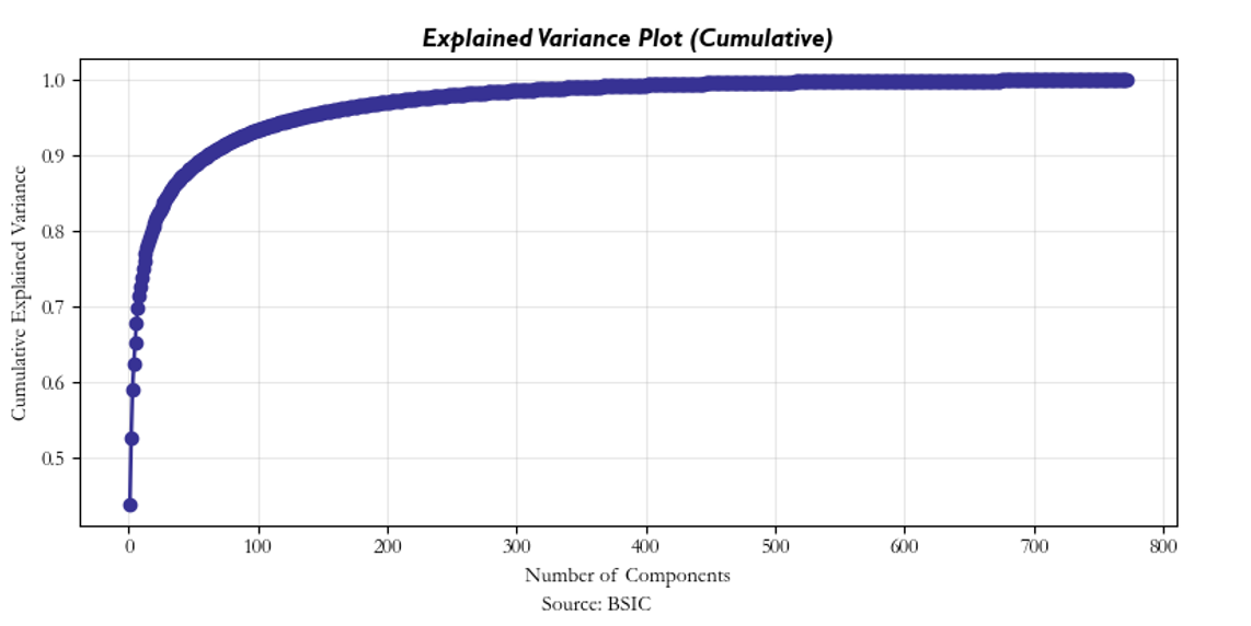
As can be seen below and above, most of the variance of the system is explained by the top 30 PCs by eigenvalue:

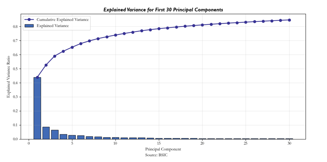
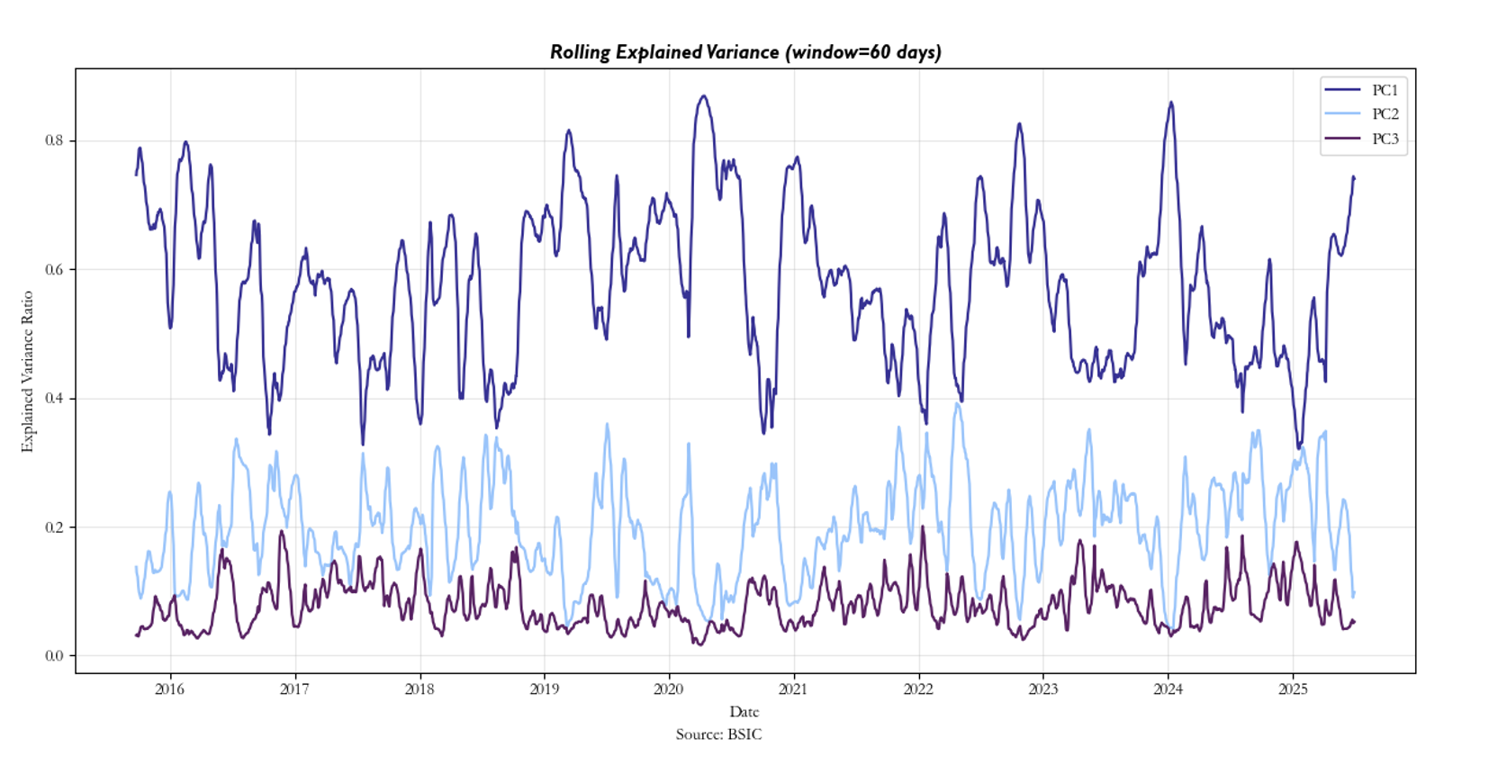
PC1 accounts for almost 45% of variability and represents global market risk factor, PC2 most likely reflects regional risk factor, and PC3 is more difficult to interpret. However, PCs are not stationary through time and not even the eigenvectors’ components are so. With a window of 60 days, the rolling variance impact of the top 3 PCs is spread out. This is certainly a caveat to the strategy, and it is our belief that the reasoning for this instability is most likely due to regime shifts as well as the dynamic nature of ETF’s exposures. In particular, if an ETF is rebalanced on a daily basis such that it now includes stocks which have lower or higher beta to the rest of the market, this can significantly impact the initial PCs’ explanatory power of total variance over a long enough time horizon. The results can be seen below:

Each return can be decomposed into a systematic component explained by common risk-factors and a residual εᵢ. Formally, for stock i,

where are the factor returns and are the loadings measuring the sensitivity of the asset i to factor j.  The residual term εᵢ represents the asset’s specific deviation from its factor implied fair value.

In the PCA approach, the factors Fⱼ are obtained as the principal components of the empirical correlation matrix of standardized returns.  Denoting the eigenvectors by
and their eigenvalues by λ₁ ≥ λ₂ ≥ … ≥ 0, the j-th factor return or eigenportfolio return is:

Hence, in our universe for each ETF we can write:

where the first 15 principal components (PC₁ … PC₁₅) explain roughly 80% of the total variance of market returns, in our universe. The eigen-portfolio weights are re-adjusted daily based on a rolling window of n days to capture PCA components (both PCs and each PC’s component) variations.

According to Avellaneda, the residuals εᵢ are modeled as mean-reverting Ornstein-Uhlenbeck (O-U) processes:

where κᵢ>0 is the speed of mean reversion, mᵢ is the long-run equilibrium level, σᵢ is the volatility of the residual, and dWᵢ(t) is a standard Brownian motion.  This stochastic model implies that deviations Xᵢ(t) (the residuals) tend to revert toward mᵢ over time, rather than drifting indefinitely.

In this setting, the residual tends to fluctuate around  with a stationary variance given by:

The s-score standardizes each residual by its equilibrium variance to measure how far it is from equilibrium in units of standard deviations:

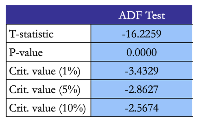
However, Avellaneda & Lee (2008) show that the mean term is 0, further supporting the assumption behind the mean-reversion nature of residuals. Then, the s-score can be approximated to:

In our universe, The ADF (Augmented Dickey-Fulley) test further supports the implication that residuals are stationary:

A strong limitation of the strategy is that it trades the asset, not the residual directly. Where the asset’s next day return is the sum of:

The trade only makes money from the strategy if the residual’s mean reversion dominates any systematic drift over the holding period. For this reason, the long-short dynamic introduced by Avellaneda & Lee seeks to enhance residual exposure via the long-short mechanism. It works like this: when a long (short) opportunity is found on one equity according to the s-score, another equity within the universe where the residual’s s-score is sufficiently positive (negative) will have the opposite position taken upon it. The idea at its core here is to neutralize market exposure via these opposite positions. Still, this approach is merely an approximation, as it’s not entirely effective at eliminating beta, and as such, we are still at the whims of systematic factors which may assert their presence over  our returns.

For the empirical implementation, we revisit the parameterization used in Avellaneda & Lee (2008). The estimation window is set to 60 trading days, which provides enough data to estimate the Ornstein-Uhlenbeck (O-U) parameters while maintaining responsiveness to changing market conditions. The number of principal components retained is fixed at n_factors = 15, capturing approximately 80% of the total variance in the cross-section of returns. Trading signals are generated using s-scores: the entry and exit thresholds correspond to:

This ensures trades occur only for significant deviations from equilibrium to mitigate transaction costs from excessive trading.

Performance measures

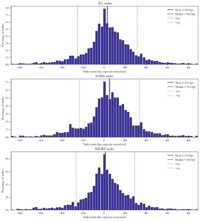
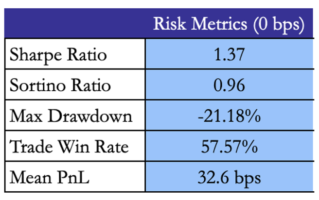
As for trading frequency, the mean holding time is 1.24 days and the strategy averages 2.38 trades per day. This makes sense given the relatively fast reversion speed of the residuals. On the other hand, our win rate and mean PnL  is 58% and is 32.6 bps per trade, respectively. Naturally, this reflects decent returns especially considering the number of trades this strategy produces.

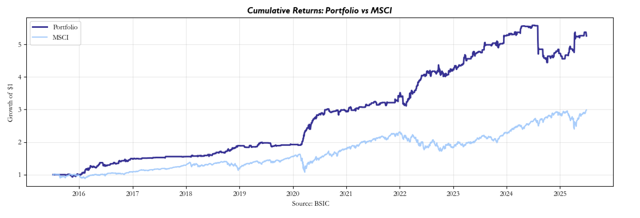
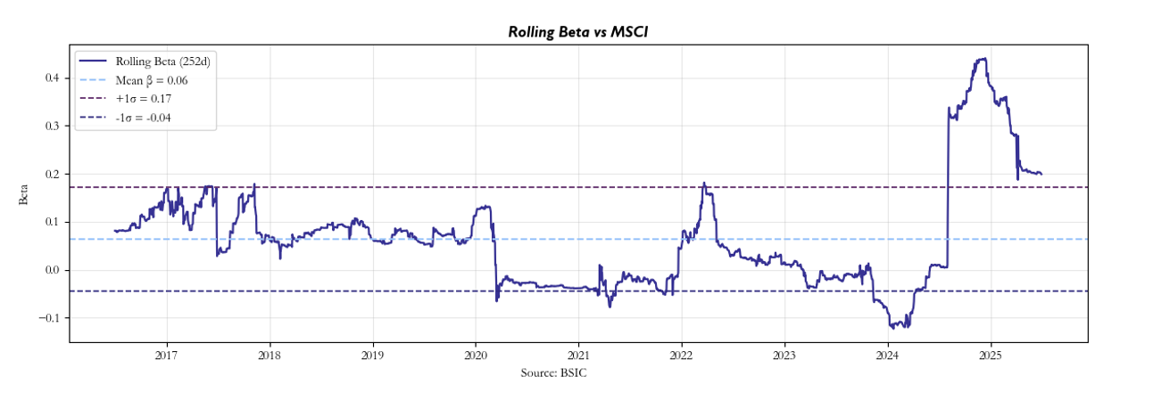
Relative to buy-and-hold MSCI (our chosen benchmark of the universe’s market), it’s clear that our strategy tended to outperform. However, the question naturally becomes: is this just beta, or are these indeed the residuals which dominated the return profile? Our attempt at addressing this issue was to compute the rolling beta, which revealed that throughout the course of the backtest, our returns have been somewhat uncorrelated. It is our view that large changes can primarily be attributed to regime shifts.

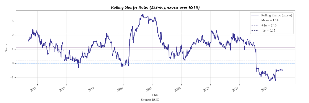
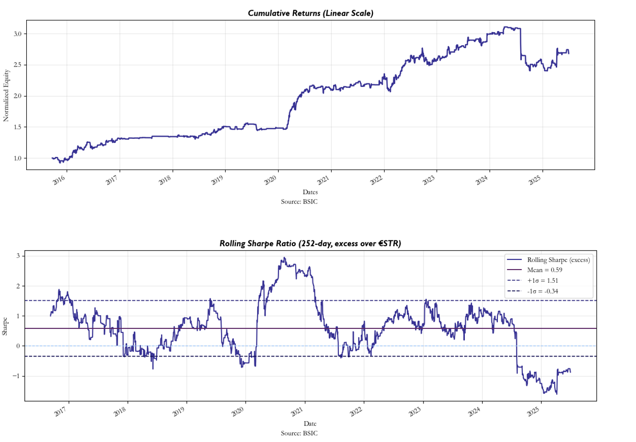
Once transaction costs are introduced, however, we see a noticeable decline in performance despite our attempts to maintain high entry thresholds, but nonetheless, our strategy maintains positive returns as can be seen below along with the rolling Sharpe:

Conclusions

The strategy rationale is that it catches residual inefficiencies in the market. It works quite well for our universe despite the caveats previously mentioned (somewhat unstable PC explanatory power, inefficient hedging of beta). After around 15 principal components, the model no longer explains fundamental or idiosyncratic structure; what’s left are mostly inefficiencies and noise which is exactly why the mean-reversion works. The strategy effectively computes, at time t-1, the return component unexplained by the principal components, which is the “inefficiency.” Since these residuals are stationary, at t > t-1 they statistically tend to revert toward equilibrium, creating a higher win rate in the direction indicated by the signal. However, when systematic returns move significantly due to large regime shifts, the model’s structure breaks down, inefficiencies stop being well defined, and the strategy’s performance becomes random. During stress regimes (2020 COVID crash, 2025 tariffs shock, etc.), factor loadings change and residual decomposition becomes unstable. Thus, the residual signal no longer isolates inefficiency. As a result, residual reverts but asset return is dominated by systematic movement. The “stat-arb” essence becomes “stat-roulette”!

Therefore, if one were to truly try and trade these residuals, we believe the following considerations must be made: firstly, one should aim to account for the dynamic rebalancing of these ETFs. For instance, decomposing equity returns via PCA and explaining variance of the ETFs as a dynamically weighted average of said returns could be an interesting way to tackle this problem. Furthermore, you could use this better interpretation of sources of beta in order to implement a more efficient proxy hedge (this limits the “stat-roulette” dilemma) which explains as much of these PCs as possible. The reason we would need a proxy hedge is of course that perfectly hedging these exposures in such a large universe would be incredibly difficult as well as capital-intensive even with just 20 PCs. It’s all about trade-offs at the end of the day!

References:

[1] Avellaneda et. al., “Statistical Arbitrage in the U.S. Equities Market”, 2008