Exploring the Application of Kelly’s Criterion in Portfolio Optimization

Download PDF

Introduction

When managing a portfolio, the fundamental problem is to find investments with excess risk-adjusted expected rates of return. Once the manager has identified some favourable opportunities and is ready to assemble the portfolio, they still need to decide how much capital, as a fraction of the value of assets under management, to allocate to each single trade. Assigning weights to each investment in a portfolio is what position sizing is about and the related decisions can significantly impact the long run returns of the portfolio. Empirical evidence shows that most traders tend to base their portfolio position sizing on heuristic rules, subject to behavioural and psychological biases, that, obviously, do not mathematically guarantee performance maximization.

Mathematical Theory

The goal of finding a mathematical theory able to determine the optimal position sizing for a portfolio composed of investments with positive risk-adjusted rates of return includes the notion of Kelly Criterion, described for the first time by J. L. Kelly Jr. in 1956. Originally invented to optimize wager sizes for gambling games that offered a positive expected value, the mathematics behind the Kelly Criterion have been extended to handle multiple correlated positive expected value bets, like stock portfolios. Nowadays, the Kelly Criterion has been implemented in many trading and investing strategies, to the point that even world-renowned investors such as Warren Buffet and Bill Gross reported to use the Kelly method in one of its many variations.

Before diving into portfolio management applications, it is worth briefly tackling the Criterion from a general angle, and to explain the mathematics behind it. For ease of understanding, we illustrate using a simple case, coin tossing, but the underlying concepts can be easily generalized.

Consider a coin, which guarantees, at each trial, a winning probability of p, where , and therefore a losing probability of . Also, the payoff in the event of winning is equal to +1, while in case of loss is equal to -1.

Since the game has a positive expected return, in order to maximize , the expected value of the wealth after n trials, we have to maximize , the expected value of the bet at the kth trial. Thus, to maximize expected gain the player should bet all their resources at each trial, which is extremely risky and almost guarantees ruin after few coin flips. At the same time, deciding the wager aiming at minimizing the ruin risk is an undesirable criterion as well, since it would require betting nothing at every trial, making no profit at all. This suggests that the optimal fraction of the bankroll to bet at each trial f, according to Kelly, is an intermediate value with respect to the two strategies described above, or rather a compromise between f = 1, which maximizes and assures ruin, and f = 0, which minimizes the probability of ruin but does not allow the player to profit from the game.

After this consideration, we introduce Kelly’s Criterion goal, which is to maximize the expected value of the natural logarithm of wealth, where the logarithmic function represents the value of money in terms of utility^[1].

If S is the number of successes and F the number of failures, then the capital after n trials is:

Note that since: , then we have:

Which is the exponential growth rate per trial.

Turn now to the expected growth rate:

As stated above, Kelly’s Criterion consists in maximizing , which, for some n fixed, being

is equivalent to maximize .

Consider now: , setting it equal to 0, we find the stationary point

Analyzing the function further, we find that, since the second derivative of g is always negative, is the unique global maximizer for g(f), whose corresponding maximum is . Moreover, the nature of the function (shown in the following graph) shows that there exists a unique such that .

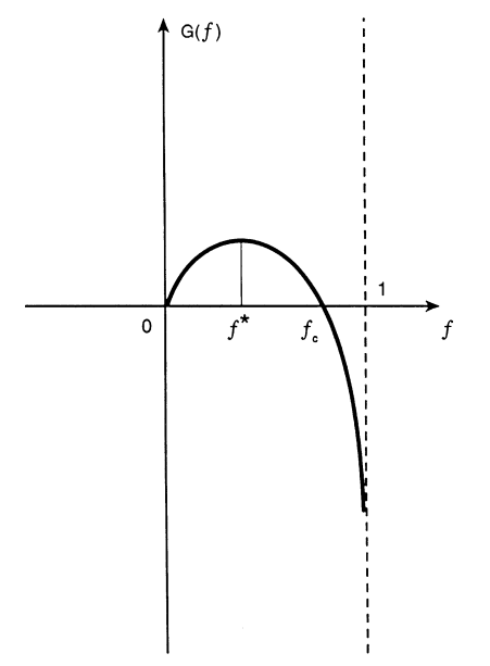
The conclusion of the problem is that, as , the player wealth unboundedly grows for every , but the optimal rate of growth is achieved as (Kelly strategy). On the other hand, whenever , ruin is almost certain^[2]; while when , the player’s wealth oscillates randomly between 0 and .

The simplest version of Kelly’s formula, that we use in binary games like coin tossing, can easily be generalized to non-binary games, allowing for partial wins and partial losses. That is:

Where b is the fraction of capital lost in case of negative outcome and a is the fraction of capital gained in case of positive outcome.

Kelly Criterion for Portfolio Optimization

In order to implement the Kelly Criterion in the realm of portfolio optimization, one must consider a variable of the formula which takes into account continuous probability distributions. This is because for a financial asset there are an infinite number of outcomes to every possible bet that can be placed.

In this case, the formula that would be derived to obtain the optimal Kelly fraction/percentage would be:

where is the mean return of the asset, r is the risk-free return, and is the volatility.

A portfolio can be optimized under the Kelly Criterion in order to form a Kelly portfolio. A Kelly portfolio maximizes the expected return of any given combination of assets in the long run, by maximizing the geometric growth rate of the wealth, which can be expressed by:

This means Kelly portfolio will have larger positions for bets which have a higher expected return.

However, a Kelly portfolio has a number of limitations, which prevent it from being the clear-cut best optimization method in most cases. These have cause numerous debates on the effectiveness of its application. Firstly, it should be noted that the first criterion to evaluate whether you should or should not use this method of optimization is determining your number one priority. In most cases, an institutional investor’s number one priority is often maintaining a certain risk-level, not maximizing returns regardless of risk level, in order to avoid withdrawal of funds for example. A Kelly portfolio does not do this in any way, which reduces its utility at an institutional level.

Also, Thorp (1971) proved that Kelly portfolios were not always mean-variance efficient, which again might discourage institutional investors from utilizing the criterion. This makes it a strategy more applicable to retail investors, who might be more willing to accept potential large short-term losses, knowing that they are maximizing wealth in the long-term. Also, Kelly portfolios are often notoriously concentrated due to the nature of calculation in the criterion, thus making them riskier in this respect, than other optimization methods such as Markowitz, or tangent portfolios.

Furthermore, Samuelson (1971, 1979) showed that a Kelly portfolio is asymptotically optimal, but not optimal in finite time, as the high leverage or position size often leads to large drawdowns, which obviously hinder performance, by adding short-term risk. This is why Kelly portfolios work better in the long run. Another reason why Kelly portfolios work better in the long run is simply because of Bernoulli’s Law of Large Numbers. This has been proven by Carta and Conversano (2020) with Monte Carlo simulations which show Kelly portfolios’ performance support the properties of the Kelly Criterion much better at 40,000 trades than at 1,000 or 100 trades.

One way that these risks and disadvantages can be mitigated, is by implementing fractional Kelly as the criterion for the portfolio optimization. Fractional Kelly optimization is a variation of the traditional Kelly optimization, where the Kelly value obtained is divided, usually by 2 or by 3 to obtain more conservative bet sizes. These ensure your portfolio stays in the left (safe) side of the Kelly curve even if parameters are misestimated slightly, which minimizes your drawdowns, albeit reducing your expected returns. By reducing position sizes to fractions of Kelly positions, one can include more positions in a portfolio, and thus increase diversification.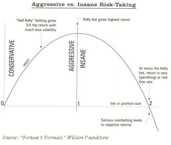

Source: Seeking Alpha

These factors, in combination with the fact that the Kelly Criterion is so sensitive to parameter misestimation, are the reason why the Kelly Criterion should be seen as the upper bound of leverage to use in each position of your portfolio, as opposed to the target amount. If the Kelly Criterion is used as a target amount for leverage with every trade, ruin is a possibility.

This can be boiled down to the fact that the strategy returns are non-Gaussian. In other words, a normal distribution greatly underestimates the tail risk of a Kelly strategy, which again highlights why a Kelly strategy carries more short-term risk than what is usually anticipated. Tail risk can be modelled more effectively with a Generalized Pareto Distribution, or other fat-tail distributions.

Another potential issue with Kelly portfolios is that the stock market contains ‘fluid odds’, meaning that the parameters of the equation needed to calculate the Kelly Criterion vary every second of every trading day. Naturally, this leads us to the fact that a Kelly strategy works best with frequent rebalancing, in order to always be in the optimal position size or leverage window. The problem with constant rebalancing is that transaction costs end up eroding the returns the strategy yields. This is a problem which is often overlooked as most Monte Carlo simulations, and other methods used to back test Kelly strategies published online assume no transaction-costs.

Backtest of the Partial Kelly Portfolio

In order to backtest the strategy, we proceed with a simple implementation of a Python script of the Kelly criterion on a portfolio of all the components of the S&P 500 and compare its performance to both the actual index as well as the SPXEW (the S&P500 index that just has equal weighting for all of its components). The formula was fed data from 2016 and the portfolio was tested on the period going from 2017 to the end of 2022.

To do this, it is needed to first calculate the expected daily returns for each stock as well as their covariance based on their 2016-2017 window performance and compute the average risk-free over the same time (assumed to be 1.84%). Based on the data we then found the Kelly weights for each component by optimizing the quadratic formula for the Kelly criterion (which can be found on this GitHub Repository). Once obtained the weights, we proceed to add further constraints to constraint any leverage, as well as adding the assumption of no short selling. We can call this strategy a partial Kelly. This results in one of the many variations which reduces potential returns but makes up for it by reducing risk more than proportionally. This allows for a strategy that mitigates the shortcomings of a full Kelly strategy, like the fractional Kelly explored earlier in the article.

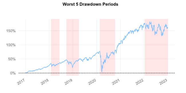
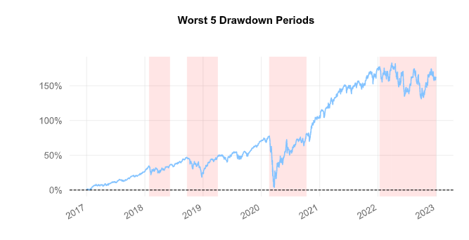
Since the trade is always open, there was no need to model turnover and transaction costs are negligible. As per the report below, the long-only partial Kelly achieved a Compounded Annual Growth Rate of 17.4%, generating an outperformance during the 2017-2022 period with respect to the SPX of more than 6.24% and 7.09% with respect to the SPXEW. It also boasted a more attractive Sharpe ratio (0.84) as well as a much shorter duration of Drawdown days (at 275 days compared to 360 of the SPX and 359 of the SPXEW). However, as explained in the shortcomings of the Kelly criterion above, a higher long-run expected return comes at the cost of higher volatility and a bigger maximum drawdown during all the negative returns periods considered. (-41.65% compared to the SPX’s -33.72%).

We expected the performance of the partial Kelly S&P500 to increase using a rolling strategy, possibly updating the sizing of each stock every quarter or even every few days in such a way to avoid having the index deviate too much from the optimal position sizing, however this would come at the cost of much higher transaction costs.

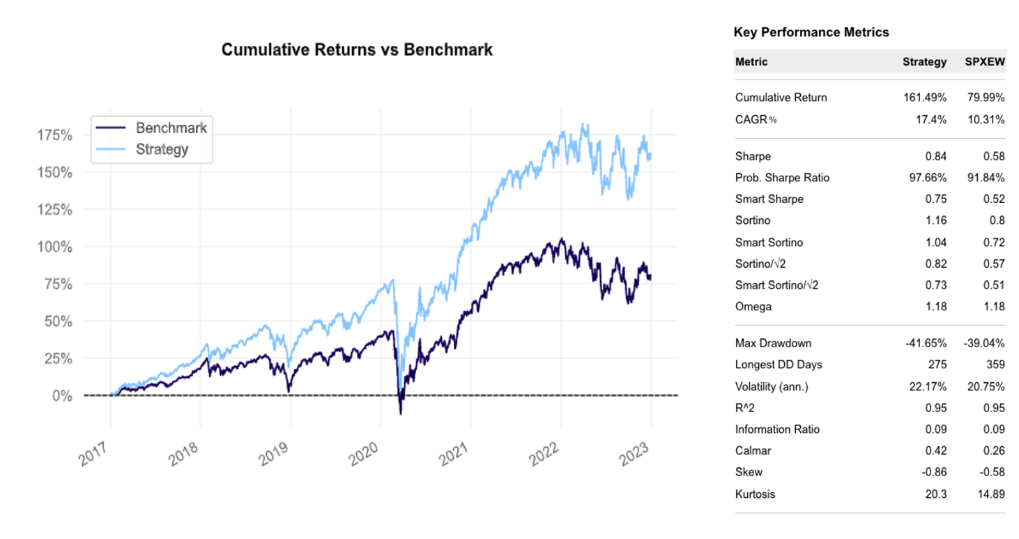
Kelly-weighted S&P 500 vs SPXEW
Source: Bocconi Students Investment Club

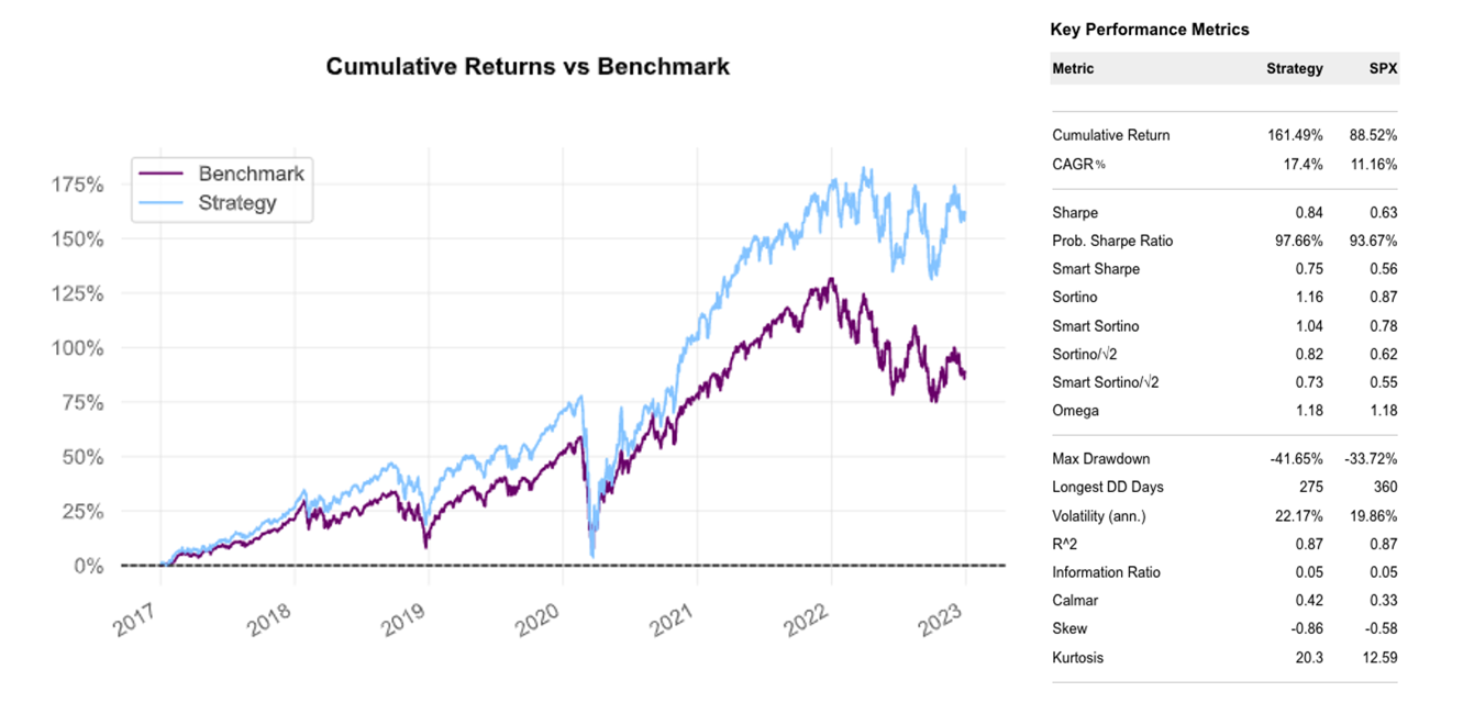
Kelly-weighted S&P 500 vs SPX
Source: Bocconi Students Investment Club

1. The nature of the logarithmic function optimally models the utility of money: the slowing pace of increase as x goes to +∞ well represents the decreasing marginal utility of the marginal dollar, while, as x goes to 0, it plummets rapidly to -∞, which symbolizes the disutility associated with going bankrupt.
2. Since f<1, it is technically impossible for the player to reach total ruin. Henceforth, here ruin’s meaning is that for some ε >0 arbitrary small: