Introduction
Convertible bonds are a unique way of raising capital which allows investors to convert the security into a predefined number of shares of common stock given by the conversion ratio. Convertible bonds have a long history, dating back to the 19th century when American railway firms were seeking to raise cash. Due to the difficulty in obtaining capital through the typical issuance of shares or bonds, convertible bonds emerged as a very appealing alternative financing option for both corporations and investors. The right to convert the bonds gave investors all the upside of equity to benefit from rising equity prices in the rapidly growing American economy, whilst giving them the downside protections of debt such as receiving coupons and the ultimate repayment at maturity. Meanwhile for companies, it offered them a cheaper method of financing operations than traditional stocks or bonds.
The market for convertible bonds was long thought to be reserved for small and medium-sized businesses. This view shifted in the 1980s when IBM, which despite still holding a triple-A credit rating, issued a $1.25bn convertible bond to finance a corporate takeover, thus benefiting from lower interest payments compared to those on conventional corporate bonds. Even though convertible bonds have historically been favoured by younger biotech and technology companies that find it difficult to access traditional bond markets, more established businesses have also jumped into the market as rising interest rates from the Federal Reserve have increased borrowing costs, even for investment-grade companies. In fact, 2023 saw a boom in convertible bond issuances, with $48bn worth of debt being issued representing a 77% growth from the year before according to data from LSEG. The rationale underlying this surge becomes apparent when contemplating the prevailing interest rate environment; when interest rates are at 0%, traditional debt financing is already very cheap eliminating the necessity to incentivise investors with conversion opportunities in exchange for reduced interest rates. Contrastingly, when rates are at 5%, issuing a convertible with a 2% coupon yielding substantial cost savings compared to a standard bond with a 7% coupon. With a significant maturity wall looming in the next two years, we can expect convertible issuances to stay extremely popular, presenting savvy investors unique opportunities for arbitrage.
Arbitrage in the convertible bond market has a slightly shorter, yet still storied history. In 1962, Ed Thorp, an MIT professor of mathematics wrote his inaugural book “Beat the Dealer” on blackjack, introducing the world to his Hi-Lo card counting system. Ed Thorp was able to turn the house edge against them at the blackjack table by using basic strategy and altering bet sizes according to the true count and the Kelly Criterion. Naturally, Ed Thorp was targeted by the casinos as soon as they were able to fire card counters, and consequently turned his attention towards another field where subjective judgement could be enhanced by computer simulation: convertible arbitrage. In 1969, he established Princeton Newport Partners, which is widely acknowledged as the pioneer quantitative hedge fund. It compounded at a rate more than twice as fast as the S&P 500 over the course of eighteen years, turning $1.4 million into $273 million without ever experiencing a single quarter of loss. Since then, many of the most renowned investors of today have drawn inspiration from Thorp’s methods and misadventures. Bill Gross, who founded Pimco and built it into the bond titan it is today, spent a lot of time at blackjack tables and setup as an investor using Thorp’s 1967 book “Beat the Market”; Ken Griffin set up his first convertible arbitrage fund at Citadel in 1990 using documents that Thorp gave him from Princeton Newport; Boaz Weinstein learned card counting in the early 90s after reading Ed Thorp’s aforementioned book, before being banned from the Bellagio in Las Vegas.
The convertible bond market represents just a small slice of the vast fixed income market with an approximate size of USD 375-400 bln. This is down from the USD 500-525 bln levels we saw during the pandemic years, characterised by record volatility and issuance levels, which further contributed to inflating the value of the market substantially. This is visible in the below chart as 2020-2021 represented some of the best years for the asset class, thanks to the rapidly changing conditions of the equity market, and companies need for urgent ans quick financing. The average daily traded volume in the last 5 years is around USD 1.84bln, another measure that has picked up 46% since the pandemic.
Below is the chart of the BCS5TRUU index, an unhedged index for a basket of USD liquid convertibles bonds, >$500MM only. It can be used to gain an overview of the overall performance of convertibles in the USA in the given time period.
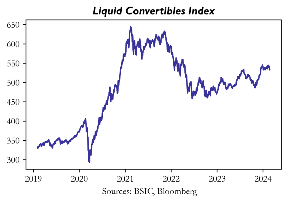
As visible from the above graph, 2020 and 2021 were record years for convertible bonds as the BCS5TRUU index saw a 100% increase in this period. The reasons for this mega performance were multiple: The macroeconomic environment created by the incumbent pandemic saw stock prices crash violently at the start of 2020, which initially made convertible bonds suffer, although not as much as the corresponding equity securities. This is due to the bond floor characteristic of convertibles. However, the extreme volatility seen in this frame contributed greatly to these returns. The S&P 500 grew 70% in the 12 months following the Covid crash. 2020 was also a record year for issuance. Between 2020 and 2021 an estimated USD 195 bln of convertible bonds were issued.
Convertible Bonds Mechanics
We can view convertible bonds as a straight bond plus a warrant (a call option on newly issued shares) on the underlying stock. The following chart shows a simplified example of the relationship that exists between the convertible’s value and the underlying stock price: indeed, the convertible in the graph is just a bond trading at par plus an at-the-money call option on the stock.
Due to these characteristics, convertibles are often valued using the standard Black-Scholes-Merton model, however this model fails to fully capture some peculiarities that convertibles present when compared to plain vanilla equity options. Stock is bought not for cash but for units of bonds according to the conversion ratio calculated as follows:  , indeed, as the bond price changes with time the Black-Scholes model does not provide an accurate description and therefore numerical procedures are usually implemented. Furthermore, indentures in the convertibles can add different layers of optionality and corporate bonds are exposed to bankruptcy risk as explained later.
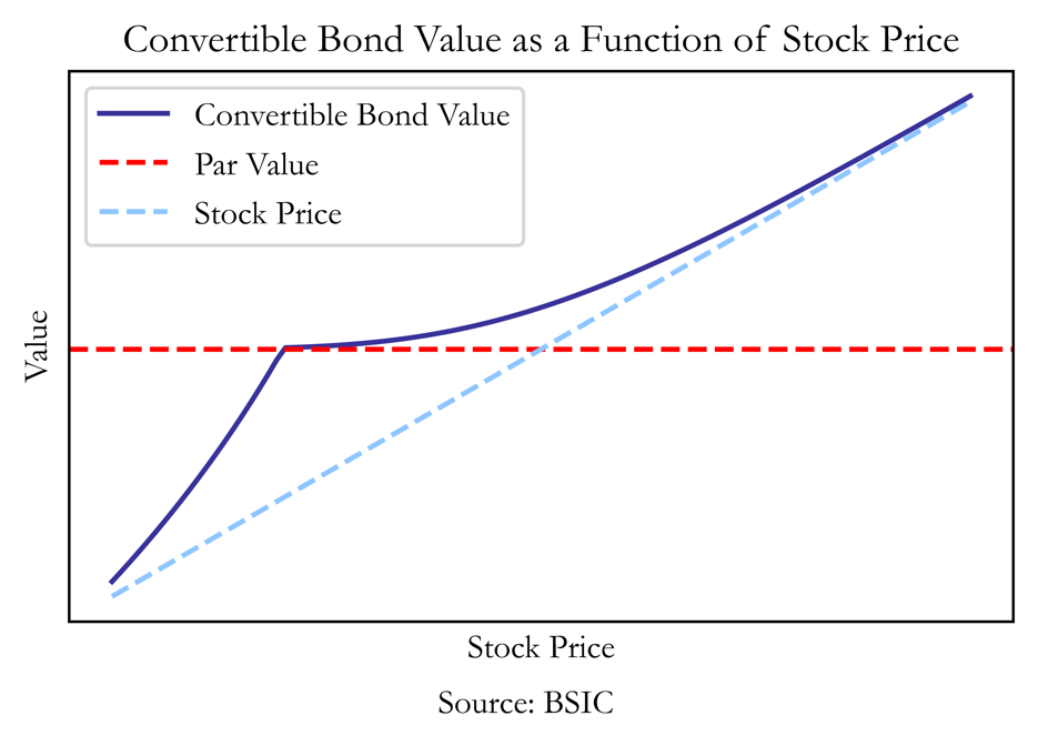
As evidenced by the graph “Convertible bond as a function of stock price” we can see the features the bond has that make it similar to both equity and to traditional debt. We can also distinguish from the nature of the curve where the bonds will behave more like equity or in a more distressed scenario like a bond. The difference between the convertible bond value and the red line “Par Value” also known as the bond floor is what is known as the investment premium given that the bond is behaving like equity. As the convertible has fixed cash flows that we can discount, even without a future conversion to equity there is a certain value of the convertible when the company is not in distress. The investment premium is simply the theoretical extra value given to the bond due to its conversion feature. The blue line “Stock price” is also known as the parity level, given that the conversion premium is the difference between the blue and purple lines as it shows the premium investors are willing to pay for the conversion option. Towards the right side of the graph where the convertible is seemingly converging asymptotically to the stock price the bond is what we call “in the money” and is behaving like equity. This is when the conversion premium is low, and there is a high probability of the conversion taking place as the share price > conversion price. It’s important to note the bond is the most sensitive to changes in the underlying when it is in the money. When the bond is at the money, the stock price is close to the conversion price and the convertible is extremely sensitive to the features we mention below (Credit events, Interest rate changes and the underlying stock price), this would be the middle section of our graph. When the convertible starts converging to the bond floor the bonds are out of the money which means conversion is unlikely and there is almost no investment premium, this results in almost no sensitivity to the price of the underlying stock. In a distressed scenario, the share price will be very low which will be reflected in the value of the convertible. The convertibles value will converge back to the stock price on the left side of the graph as that is what it is expected to recover in a liquidation scenario.
There are many types of convertible bonds which offer different payoff structures, and different risk profiles. Below are the most important specifications:
Plain vanilla: These are the most common type of convertible bond; the investor has a right to convert at a predetermined price and rate at the maturity date. The bonds pay coupons normally, and have a maturity date at which the investor is entitled to the nominal value of the bond
Mandatory: The bonds provide the obligation to convert at maturity, and usually come with two conversion prices: One at which the investor would convert at a share value equivalent to par value, and another which denominates the maximum conversion price above the bond’s par value
Convertible bonds can also be classified into different categories:
High moneyness are in-the-money bonds, and thus very equity sensitive. These usually offer the best risk-adjusted returns, but also require the most leverage in order to obtain significant profits. Hybrid convertibles are close to being in-the-money and thus are very sensitive to equity volatility. Busted convertibles are out of the money and offer limited convertibility, and lastly, Distressed convertibles are out of the money, and also carry substantial default risk.
Strategy Overview
The strategy employed in a convertible arbitrage trade is rather straightforward: the trader takes a long position in the convertible security while hedging it by shorting the underlying equity. The trade is usually one-sided as convertible bonds are usually cheaper than equity, likely as compensation for their relative illiquidity compared to stocks. Pedersen (2015) and Agarwal et al. (2006) state, in fact, that hedge funds that engage in convertible arbitrage are compensated for the liquidity they provide in the otherwise relatively illiquid convertible bonds market.
The strategy relies on convertible bonds’ characteristics as it is essentially long a call option (therefore long gamma) on the underlying stock, it tends to benefit from big moves in the underlying thanks to the convex payoff of the strategy. In particular, the strategy tends to perform well both in up and down moves in the underlying: if the stock price rises the, the price of the associated convertible bond will rise more, resulting in a profitable move. Should the price of the underlying stock return to its initial value, the result would be analogous. The value of the hedge would shrink more than that of the long position of the convertibles, only under one condition although. As the bond goes further in-the-money, the hedge has to be increased, due to the higher equity sensitivity the bond has at higher stock prices. Hence, the hedge’s asymmetry is the characteristic which allows the arbitrageur to profit from the round trip. Hedges also have to be re-adjusted once the stock has returned to its initial price.
This, however, is not always true. At extremely low underlying stock prices, the position is no longer convex, as there is negative gamma coming from default risk, having the effect of a short put option. This is why large negative price shocks can be very bad for a potential arbitrageur.
Greeks’ exposure:
The trade is delta neutral, as the hedge ratio is chosen so that the stock sensitivity of the hedge equals that of the bond. This remains true as hedges keep getting rebalanced after stock price changes, as mentioned above. This arbitrage strategy has positive gamma, an element also highlighted above. This allows the strategy to benefit from both ends of the roundtrip, in other words both increases and decreases of prices of the underlying stock. The optionality of convertible bonds makes Theta in this strategy negative. If all factors stay the same, but time passes, the value of the convertible will converge to straight debt. This is because there will be less available time for big moves in stock prices, whether up or down, to make profits for the arbitrageur. This relates very closely to Vega, which in this strategy is clearly positive. Volatility is key for profitability in this strategy, as there is potential benefit from ups and downs in stock price, hence high volatility in the underlying, makes the convertible bond more valuable.
Alpha:
The possible alpha from this arbitrage comes from buying bonds which are underpriced relative to their fundamental value. This underpricing is mostly explained by three characteristics according to Argwal, Fung, Loon, Naik (2004): The implied interest rate, the implied credit spread, and the implied option price
The ideal setup for a convertible arbitrage strategy would involve the following characteristics: Buying an underpriced bond with low conversion premium, which’s underlying stock is liquid, easily borrowable and pays no dividends, as this represents a cash outflow for the arbitrageur, who is short the stock.
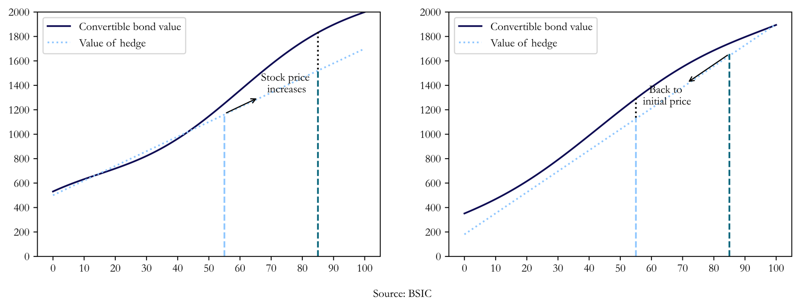
The above chart shows how, the convertible gains value more than the equity hedge on the upside and how these profits are not simply reversed when the stock price goes back to the initial level: this is caused by the dynamic delta hedging embedded in the strategy as when the stock price increase mentioned before.
Empirical Assessment
We use as a proxy for the returns of the strategy the Convertible Arbitrage index from the Credit Suisse Hedge Fund Indices, with monthly data available from 1993. We use the word “proxy” as one of the most discussed problems in hedge fund literature is the biased nature of hedge fund indices data, which could lead to unreliable results. The most notable bias discussed in the literature is survivorship bias, introduced by Grinblatt and Titman (1989) in analysing mutual fund returns, which implies that indices overlook defunct funds thus overestimating overall performance. Other sources of bias, introduced by Bianchi and Drew (2010) are backfilling bias and multiperiod sampling bias, caused respectively by the voluntary nature of reporting and by minimum survival criteria imposed by researcher. The CS indices minimize survivorship bias by removing funds only when they are completely liquidated or fail to meet financial reporting criteria.
Here we show the distribution of monthly returns on the index based on 362 observations from December 1993 to January 2024, and compare it to a normal distribution with same mean and standard deviation.
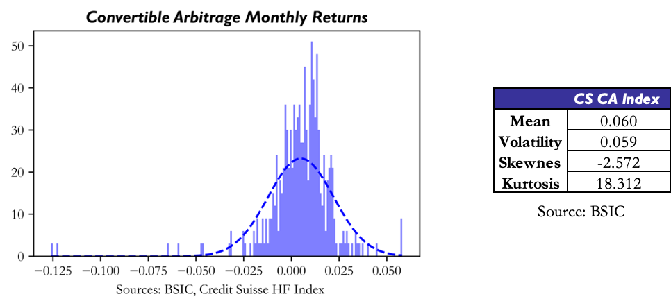
The distribution clearly shows non-normal behaviour with considerable kurtosis, consistent with the underlying strategy’s payoff structure. The strategy does, in fact, make small profits on average (and rather consistently), but is then exposed to the negative gamma introduced by default risk caused by big down moves in the underlying price.
We now proceed by analysing the factor exposures of the strategy to see if the strategy can indeed be called “arbitrage” or whether it is just explained by risk premia exposure. As mentioned before, the strategy’s profits can, at least intuitively, be explained as compensation for liquidity risk. Our aim is now to investigate if exposures to the liquidity factor of Pastor and Stambaugh (2003) and to the Fama French (2015) 5 factors do indeed explain the returns of the strategy. To this end we regress the monthly excess returns (monthly returns minus the FF5 “rf”) of the CS index on the FF5 factors and the traded liquidity factor.
We report here the results obtained in the regression:
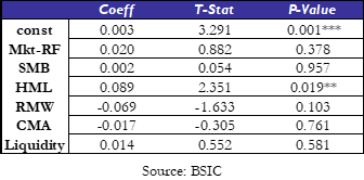
As shown by the previous table, the Fama French five-factor model plus the traded liquidity factor fails at fully capturing the returns of the convertible arbitrage CS index. The strategy yields, in fact a statistically significant (at 1%) alpha of 0.3% per month with HML as the only significant (at 5%) factor. Therefore, we conclude that, net of the biases discussed that are inherent in the data available, the strategy indeed deserves its name.
As a final step, we compare the performance of the convertible arbitrage index with the one of the liquid convertibles index introduced before over the common sample starting in 2019.
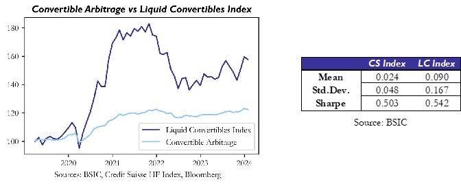
Despite the stellar performance of liquid convertibles in the US in 2020, driven by the factors previously analysed, the convertible arbitrage index was able to deliver a similar Sharpe Ratio (0.503 vs 0.542) thanks to the incredibly low volatility of the strategy, barely 4.8% annualised.
Key Characteristics
Another important thing to note are the different features of the bond which make it harder to analyse, apart from Callability that we have already discussed there is also:
- Putability – the bond holder can give the convertible bond back to the issuer at a predetermined amount called the put price
- Contingent Conversion – in the contingent conversion periods there is a restriction on the conversion, the investor cannot convert the bond into shares unless the equity price is higher than a contingent conversion threshold
- Soft Callability – in the periods when soft callability applies the issuer is restricted from calling the bond unless the underlying equity trades above a certain threshold
All these different features are very important and must be kept in mind while building a pricing model to properly analyse the security.
As previously mentioned, the extremely low volatility of the strategy due to its market neutral nature makes determining the price of a convertible bond difficult and identifying candidates for a successful arbitrage opportunity even harder. The main features that affect the price of the bond are its sensitivities to high interest rate, the credit rating of the bonds issuers and the underlying stock price. By isolating two of the 3 factors the arbitrage opportunity presents itself to invest in one of the three drivers at an interesting entry point.
The first concern that arises while selecting candidates is liquidity. Convertible bonds are notoriously illiquid assets particularly when compared to the stock in the company one is analysing, which is why the first good metric for a successful arbitrage opportunity, is high liquidity in the convertibles market. By focusing on larger publicly listed companies one can find a plethora of corporate bonds whose volume makes trading the securities easier if an arbitrage opportunity were to arise.
Another impactful metric on convertible bond pricing is their sensitivity to interest rate swings. Although this can be used to the trader’s advantage by buying the bond when they expect interest rate to decrease (selling the bond when they expect interest rates to increase) and hedging against the move in rates to generate profit when the bonds increase in value (decrease in value). It is also important to note that the interest rate risk is an issue that needs to be mitigated through financial instruments like derivatives. It’s important to understand the concept that the exercise price is dependent on the investment value which is negatively impacted by a rise in interest rates. A tool which we can measure to analyse the convertible bonds interest rate sensitivity is its duration given by the equation:

Where C = conversion value & I = investment value
The profit opportunity lies in the correlation between a change in interest rates and how much this moves the convertible bond relative to the underlying stock. The S&P 500 and the broader equity market have an implied correlation with interest rates that is negative, this causes the stock price to drop following an increase in interest rates. This negative correlation tends to lower the value of the convertible bond more than the equity and the same is true on the flip side (A positive correlation will increase the value of the convertible). On average the shift when moving from a correlation of 1 to -1 in the price differences in the convertible bonds is between 10-15% which presents an interesting opportunity.
Lastly, another important note is the impact of the issuers credit rating on the value of a convertible bond as evidenced by the monotonic nature of the bond. In distressed scenarios it’s important to hedge the convertible bond with instruments like a credit default swap to protect the downside scenario.
All of these important features to note point to the fact that a good candidate for convertible bond arbitrage will be a highly liquid large cap company that has many of financial instruments available at the trader’s disposal to hedge one’s position while investing.
References
[1] Pedersen, L. H., “Efficiently Inefficient”, 2015
[2] Agarwal, V., Fung, W. H., Loon, Y. C., Naik, N. Y. “Risk and return in convertible arbitrage: Evidence from the convertible bond market”. Working paper, Georgia State University and London Business School, 2006.
[3] Bianchi, R. J., Drew, M. E., “Hedge funds: Attrition, biases and the survivor premium”, 2020
[4] Grinblatt, M. and Titman, S., “Mutual fund performance: An analysis of quarterly portfolio holdings”, The Journal of Business, 1989
[5] Balázs Mezofi “Convertible Bond Pricing”, SolvencyAnalytics.com, 2015
[6] Igor Loncarski, Jenke ter Horst and Chris Veld “Convertible debt issues and convertible arbitrage – issue characteristics, underpricing and short sales”, 2006


0 Comments