How a CAT (bond) protects you from natural disasters

Download PDF

Introduction

Catastrophe bonds (CAT bonds), also called “Act-of-God” bonds, or “cat-in-the-box” bonds, have emerged as a compelling investment strategy, particularly highlighted by their performance in 2023, where they generated the best returns (+19.69%) of any alternative investment strategy, according to Preqin. These instruments are key for the insurance and reinsurance industries, allowing for the transfer of risk of catastrophic losses to investors. In return, investors accept the potential of losing their capital against the prospect of outsized profits if predefined disasters do not occur.

The attractiveness of CAT bonds has been significantly bolstered by increasing concerns over extreme weather events driven by climate change, coupled with the inflationary pressures on rebuilding costs post-disasters. This was evident in the aftermath of Hurricane Ian, which led to a record issuance of cat bonds in 2023, totalling $16.4bn and pushing the market to an unprecedented $45bn. Investors demanded higher returns for taking on these risks, with spreads reaching new highs. Moreover, in 2023 the market also saw the introduction of cyber-catastrophe bonds addressing the growing threat of cyber incidents, which corporate executives rank among their top external fears.

This article serves as an introduction to catastrophe bonds, offering insights into their fundamental aspects, a straightforward pricing example for an earthquake bond, and concluding with key statistics and future perspectives on this niche family of securities.

Brief History

CAT bonds are the most common type of insurance-linked securities (ILS), which are financial instruments that transfer insurance risk to capital markets. Insurance-linked securities, particularly CAT bonds, are accessed mainly by institutional investors looking for high returns that are essentially uncorrelated to traditional financial markets.

The market for CAT bonds started to develop in the mid-1990’s, following Hurricane Andrew and the Northridge earthquake, and has since rapidly grown following Hurricane Katrina (2005) and the financial crisis in 2008. The theory behind CAT bonds was developed by a group of professors at the Wharton School seeking to explore new ways of insurance against natural catastrophes. The first ever CAT bond was issued by Hannover Re in 1994, and in the following years AIG, USAA, Swiss Re and St. Paul Re followed. The CAT bond market grew steadily between 1997 and 2005, with yearly issuances of $1.2bn. A considerable surge in demand for CAT bonds occurred after Hurricane Katrina hit the coastlines of Florida, Louisiana, and Mississippi, causing $62bn in insurance losses. During the 2008 financial crisis the flow of capital towards ILS decreased significantly but resumed post-crisis, doubling the market-size in the following 8 years. Today the CAT bonds market is valued at $45bn and is growing at a CAGR of 10%.

CAT Breeds

An important distinction is necessary to better understand the types of issuances: the CAT bond market is split into two main categories, single-peril, and multi-peril bonds. Single-peril bonds transfer the risk of one single catastrophic event happening, whilst multi-peril bonds are a form of insurance against several events. The first are usually preferred by investors who wish to construct their own risk-adjustment strategies to manage their portfolio; the latter on the other hand are commonly chosen by sponsors who aim to cover as many perils as possible whilst reducing transaction costs.

Multi-peril bonds, both in the USA and internationally, constitute 48.7% of issuances, whilst the rest are single-peril bonds covering mainly earthquakes, wildfires and hurricanes and floods. Such bonds are the most common given the devastating nature of natural catastrophes. However, also different categories of CAT bonds are emerging in the marketplace, the most interesting ones being pandemic bonds, that are used to tackle global sanitary crisis’s, cyber-security bonds (which are extremely recent, given the first-ever deal struck in Q4 2023), terrorism bonds and extreme mortality bonds (EMB). EMB’s are high-yield debt instruments that look to mitigate insurance risk if a catastrophe involving a significant number of deaths were to happen. EMB’s offer a solution to companies wanting to avoid the costs of insuring numerous lives and instead benefit investors with high returns and the low probability of losing their principal. Some EMB’s require mortality rates to rise to 20-40% in a specific region before investors lose all their capital. To put into perspective, that would equal mortality rates observed during the Spanish flu of 1918.

CATs & SPVs

Typically, CAT bonds are structured in the following way:

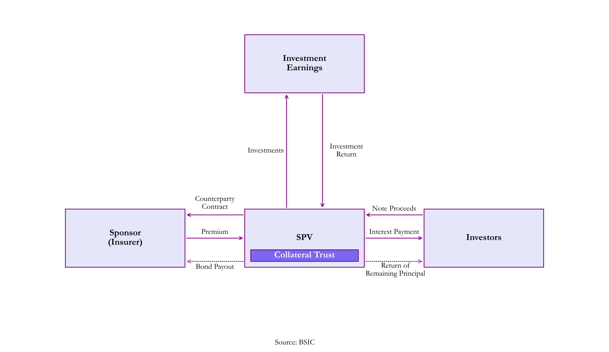
Source: BSIC

The sponsor is defined as the entity who seeks to transfer a catastrophic risk off its balance sheet directly to the capital markets. Usually, the sponsor is an insurance or reinsurance company, but other entities may also issue CAT bonds, such as large corporations (e.g., the case of Quake Bonds issued by the owner of Tokyo Disneyland), sovereign nations (e.g., the case of Chile), and supra-national entities (e.g., the Pandemic Bonds issued by the World Bank).

As we can see from the figure above, at the heart of every CAT there is an SPV. The SPV is set up in a way that it is bankruptcy remote, so that is protects both the sponsor and the investors from each other’s credit default risk. The SPV is fundamental as it:

• Sells protection against potential losses from catastrophes via a reinsurance contract, also called a cat swap.
• Issues CAT bonds to raise capital from investors who are willing to bear the catastrophe risk in exchange for a higher expected return.
• Invests the capital raised in safe and short-term securities (e.g., U.S. Treasury Bills) held in trust accounts.

As investors bear the risk, they are compensated through regular coupons, consisting of variable interest rate plus a spread component, so we can see CAT bonds as floating rate notes that have minimal duration risk. Coupons are in turn financed through the reinsurance premiums paid by the sponsor to the SPV. In case the pre-specified trigger event occurs during the term of the CAT bond, the reinsurance claim is made by the sponsor, which receives the full/partial principal from the liquidation of the securities by the SPV, leading to a full/partial loss borne by the investors (note that not all CAT bonds have a binary trigger for the loss of principal, so a bond may be only partially impaired if the trigger event occurs). Instead, if the specified event covered by the contract does not happen, the principal is fully returned to investors.

Most CAT bonds have an “Extension Period” clause, which gives the sponsor the optionality to extend the maturity of the bond when a qualifying event has occurred, but the ultimate loss in not yet known. This extension of the maturity allows the sponsor to calculate the real impact that the catastrophic event had on its balance sheet. This mechanism ensures that investors do not prematurely redeem their investment before the full extent of the bond’s obligation towards the covered losses is clearly determined. Note that an extension spread is paid over such period. Finally, after the “Extension Period”, or at maturity, investors receive the remaining principal, netted out of payouts to the sponsor.

Triggering a CAT

As we mentioned earlier, the trigger of a CAT allows us to determine whether or not a payment should be made to the sponsor. The trigger generally comes in four main flavours:

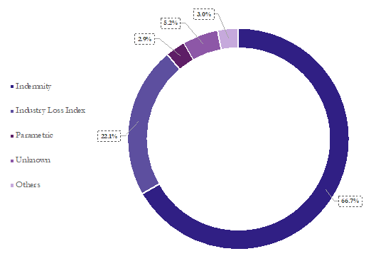
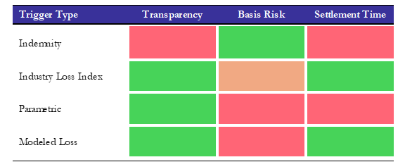
Indemnity trigger – a widely favoured mechanism, as we can see from figure below, in 2023 2/3 of the CAT bonds outstanding had an indemnity trigger. It is designed to activate payouts based on the actual insurance losses experienced by the issuing sponsor. This trigger comes into effect when the sponsor’s losses exceed a predefined financial threshold, directly aligning the bond’s payout with the sponsor’s incurred damages. While this setup offers the advantage of providing a complete hedge against catastrophe risk, making it highly beneficial for the sponsor as it closely matches their actual losses, such trigger can be opaque for investors. Investors do not have direct visibility into the sponsor’s insurance portfolio details, and this may introduce moral hazard issues. For example, if the sponsor is an insurance company, it may adopt less stringent underwriting and claims-handling standards. Another issue with indemnity triggers is the lengthy payout process, since the process of verifying received claims and loss reporting before releasing funds can delay the notification to investors about the impact on their principal.

Industry loss trigger – such trigger activates based on the total insured or economic losses experienced by the broader community, rather than the losses of the insurers themselves. It sets off when aggregate losses surpass a predetermined financial threshold. The calculation of aggregated losses is typically conducted by an independent third-party, which gathers and compiles loss reports into an industry loss index. This method effectively mitigates the moral hazard problem, as payouts are not directly tied to the individual insurer’s claims handling or underwriting standards. However, it introduces basis risk, meaning there might be scenarios where the cat bond does not trigger despite the sponsor incurring significant losses. Furthermore, collecting and aggregating data post-catastrophe is a time-consuming process, which can delay the determination of whether the bond’s trigger condition has been met.

Parametric trigger – it offers a high level of transparency for both investors and sponsors while effectively eliminating the moral hazard issue. This trigger mechanism is activated based on specific, measurable characteristics of the catastrophe, such as the magnitude of an earthquake or wind speed in a hurricane, once they exceed predefined thresholds at pre-determined locations (measurement stations). Such clear and objective criteria ensure swift payout processes, greatly benefiting recovery efforts by providing timely financial resources. Nevertheless, the parametric trigger introduces basis risk for the sponsor, since the measurable characteristics used to trigger the bond may not perfectly align with the actual insurance losses experienced. Consequently, there could be scenarios where significant losses incurred by the sponsor do not result in a payout from the CAT bond, or the payout does not fully cover the losses.

Modeled-loss trigger – this trigger was once a feature in the catastrophe bond market, functioned similarly to indemnity triggers but with a significant distinction: it relied on third-party modelers to estimate the sponsor’s projected losses when certain loss levels were reached. This method aimed to streamline the payout process by utilizing sophisticated models to quickly assess and estimate future losses, potentially accelerating financial support to the sponsor. However, like the parametric trigger, the modeled loss trigger introduced basis risk, where the estimated losses might not align perfectly with the actual losses experienced by the sponsor. Despite its potential for faster payouts compared to traditional indemnity triggers, this type of trigger has phased out of use in the catastrophe bond market.

Source: BSIC, Artemis (2023)

Source: BSIC

Note that other types of triggers exist. For instances, the Mortality Index is adopted in the case of Extreme Mortality Bond (EMB), but there are also CAT bonds which use hybrid triggers, meaning a combination of more than one trigger. In addition, CAT bonds may also be separated into tranches, which either exhibit different risk-return profiles or vary in terms of trigger mechanism.

The design of the payout structure in case of trigger of CAT bonds can also be customized. Usually, we distinguish between proportional payouts vs binary payouts. Proportional payouts are designed to vary according to the severity of the catastrophe, and a full loss happens when the underlying insurance losses hit the “exhaustion point”. On the other hand, binary payouts adopt an “all-or-nothing” strategy, where the occurrence of predefined trigger conditions results in a full transfer of the principal to the sponsor, irrespective of the event’s severity beyond the trigger threshold.

Pricing a CAT

In this section we will present a simple model to price earthquake bonds for the city of San Salvador in El Salvador through historical simulations, following the model for the spread of CAT bonds introduced by Lane (2003). Indeed, this will be an indicative example of how one can go about modelling the spread on CAT bonds using few parameters and the model can be extended to include more and more parameters or to include more sophisticated techniques. In this article, however, we aim to present to the reader how one could structure an analysis for a similar problem.

The first thing that we need to do to this end is to get earthquake data: we obtained data from 1/1/1900 to 1/1/2024 through the US Geological Survey API for earthquakes within a 500km radius from San Salvador. We plot here the observations on a map, highlighting the 10 strongest earthquakes and plotting circles of 50-100-150km of radius that will be used later in our analysis:

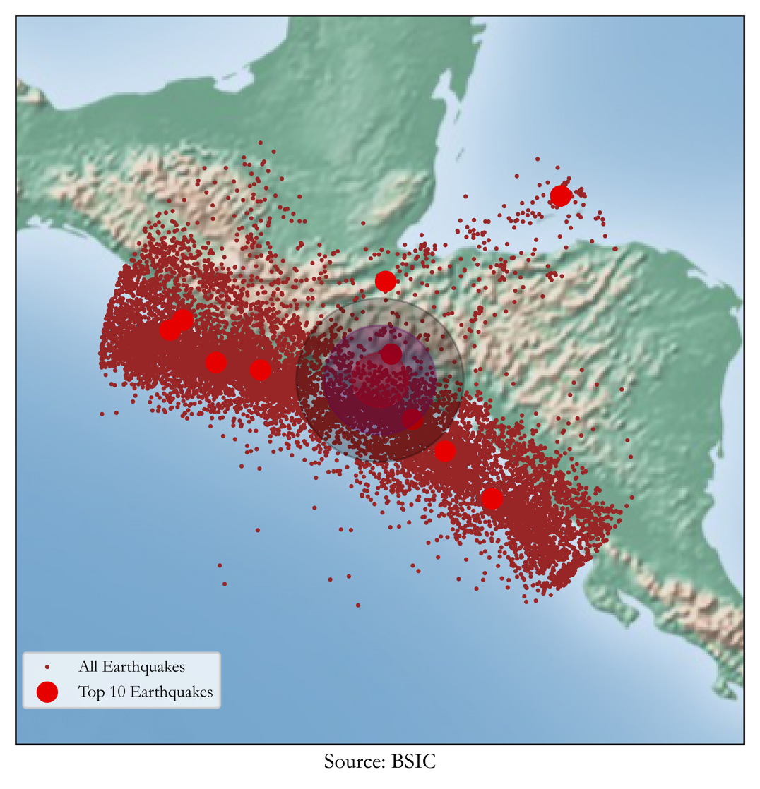
As can be seen, pricing CAT bonds for this region can be useful as it lies on a highly seismic area, with 11,854 registered cases in the analyzed dataset since 1900 with an average magnitude of 4.42 and depth of 56.41 km.

In our analysis, the aim is to compute a spread for the bond over a reference rate (when the model was presented this was Libor) based on the expected loss caused by the earthquakes. Indeed, to calculate the expected loss we will use the historical data to calibrate the parameters of the historical simulations we will run to get to the spread through the formula presented by Lane (2003):

Where the spread is therefore calculated as a power law where PFL is the probability of first loss, CEL is the conditional expected loss computed as the where EL is just the weighted sum of the losses encountered. In this Cobb-Douglas style equation, frequency and intensity of losses are traded off according to the parameters . In particular, for this example we will use the parameters obtained in Lane (2003): , otherwise the parameters can be estimated empirically.

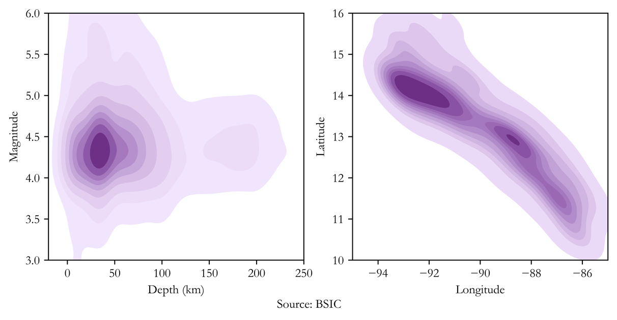
We will now proceed in analyzing the parameters we will use to price our CAT bond: we need to understand the distributions of location, magnitude, and depth of the earthquakes in order to be able to run a historical simulation for each parameter and compute expected losses for our bond. The chart below shows how depth and magnitude correlate, as well as the geographical areas more affected: a darker shade of purple indicates points where most observations are located, both geographically and in terms of depth and magnitude.

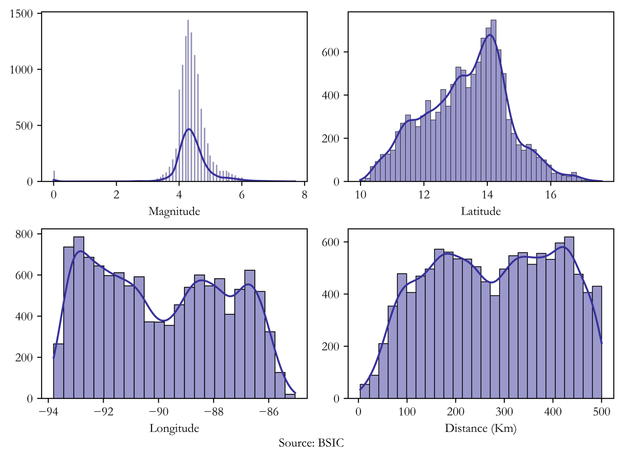
At this point, what we need to do is to calculate the distances of earthquakes from the coordinates of San Salvador, earthquake based on its latitude and longitude parameters that are directly obtained from the API. After doing that, our simulations can be run: we will simulate 1,000,000 earthquakes from their empirical distribution of distances and magnitudes, represented in the following chart (note that a maximum distance of 500km happens by construction as we only considered earthquakes within this radius):

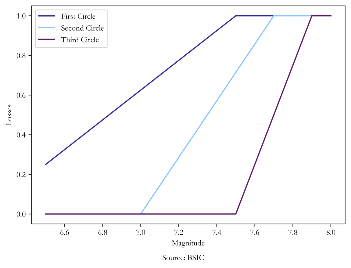
Now the last step is to characterize every distance and magnitude with a certain degree of loss, to this end we use a simplistic approach based on a linear representation based on which of the circles drawn on the map the earthquake happens: in particular, we use a linear increasing function that increase differently from 0 to 1 for each circle and for each magnitude. Indeed, the circle with the lowest radius (50km) will suffer more severe losses than the other circles (100km and 150km) for lower magnitudes. Finally, we consider only magnitudes above 6.5 magnitude in order to ensure only from catastrophic earthquakes, as the name of the bonds indicates.

Now we have all the pieces, and we are able to find the spread to price our bond: in this particular case, we will price a bond that insures only events happening within the first circle (i.e., within 50km from San Salvador) and having a magnitude greater or equal to 6.5. Note that considering also the other circles would not require any complication as losses would be additive and therefore .

Assuming a bond issue of $1bn, after running 1,000,000 simulations we obtain an expected loss of 0.45% calculated as the average loss level from the previous chart for the first circle across the simulations by applying a “stress” parameter of 5% (i.e., by increasing simulated magnitudes by 5%). Furthermore, we computed the probability of first loss as the historical probability of having earthquakes within the first circle above 6.5 magnitude, obtaining PFL = 1.9%. We are finally able to price our bond at a spread of 4.057% over the reference rate according to the formula previously presented.

Historical Performance

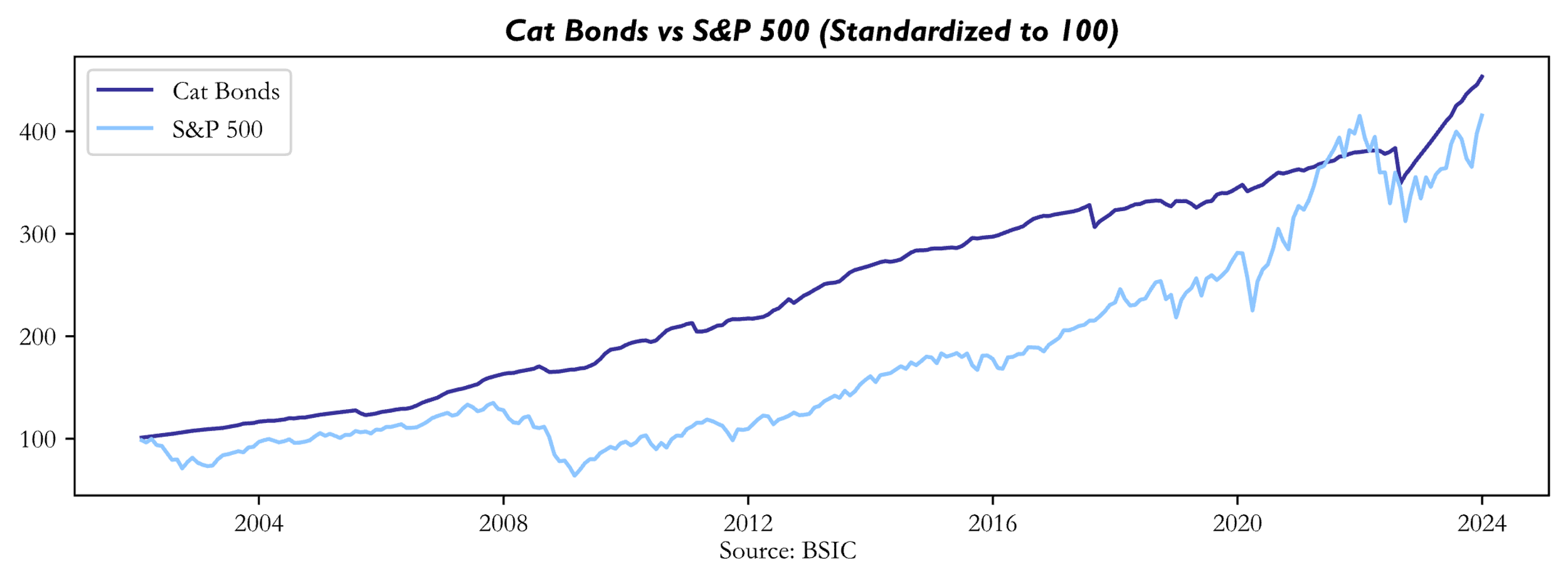
For this section we considered the data taken from Bloomberg on “Swiss Re Cat Bond Total Return Index” (SRCATTRR), which tracks the total rate of return for all outstanding USD denominated cat bonds. The index captures all rated and unrated cat bonds, outstanding perils, and triggers. We considered monthly data for the index, starting from 01/01/2001 until 31/12/2023. Indeed, such an index will smooth the rare but large losses of individual bonds, that will have huge negative returns when they are triggered.

The below chart shows the performance of the CAT Bond Index compared to that of the S&P by standardizing the initial value for 2001 at 100 for both indices. The Cat Bond index reached an all-time high in December 2023 by displaying a growth of 449.67% compared to the S&P’s 415.46%.

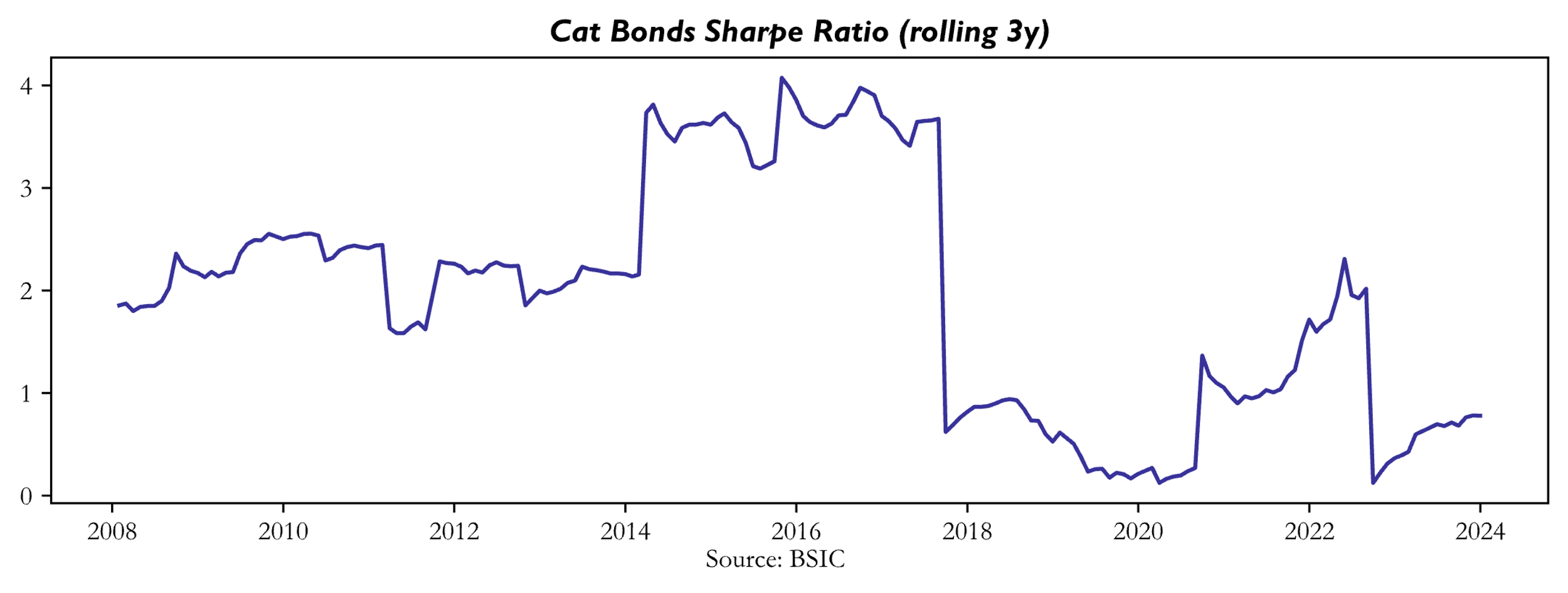
The outstanding returns of the index were coupled with an even more incredibly low measure of annualized standard deviation of 3.72% compared to an average return of 6.92%. This incredible performance is coupled with a very high Sharpe ratio, with excess returns calculated over the risk-free rate provided by the Fama-French dataset.

The below chart reports a measure of 3-year rolling Sharpe ratios that reached incredible levels of ≈ 4 in 2014-2018 where the series was growing almost in a straight line. The final observation as of December 2023 was a Sharpe of 0.73

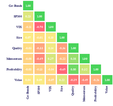
The performance was outstanding when considering its intrinsic properties, we now want to analyze how the index relates to other assets to understand whether CAT Bonds provide considerable diversification to traditional asset classes. The following chart reports the correlation matrix between cat bonds and different assets and factors.

Source: BSIC

The correlation matrix shows that the CAT bond index (first column) has very low correlations to all of the asset classes, especially to factors, with the highest correlation being with the S&P at a still quite low 23%. The analysis of the correlations brings us to wonder if the performance of CAT Bonds can be explained by traditional asset pricing factors, therefore we regressed the monthly data of our sample on the Fama-French 5 factors and we obtain the following table of the OLS estimation.

As expected from the correlation matrix, we do not get any significant betas for any factor and the only significant parameter is the constant at 0.6% per month. This confirms that an exposure to CAT Bonds can provide significant diversification and positive returns independently of traditional risk premia.

We now wish to analyze how the performance evolved over the years and especially how the performance clearly relates to the occurrence of natural disasters.

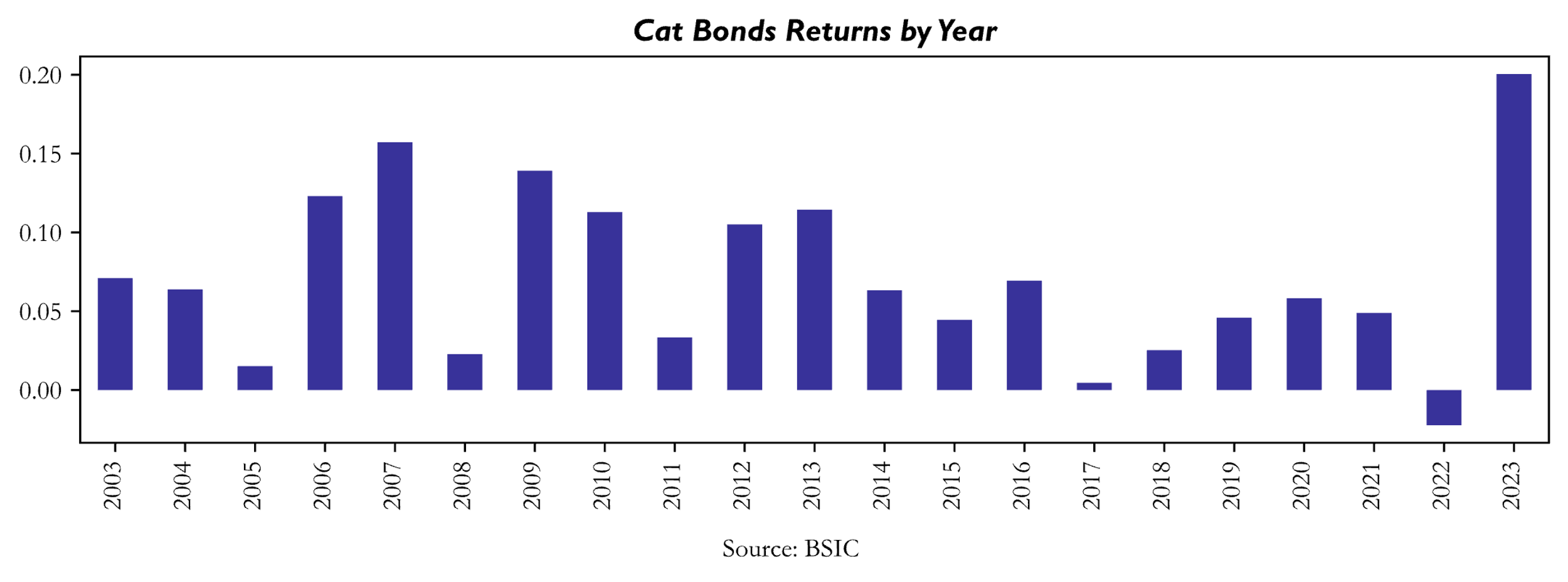
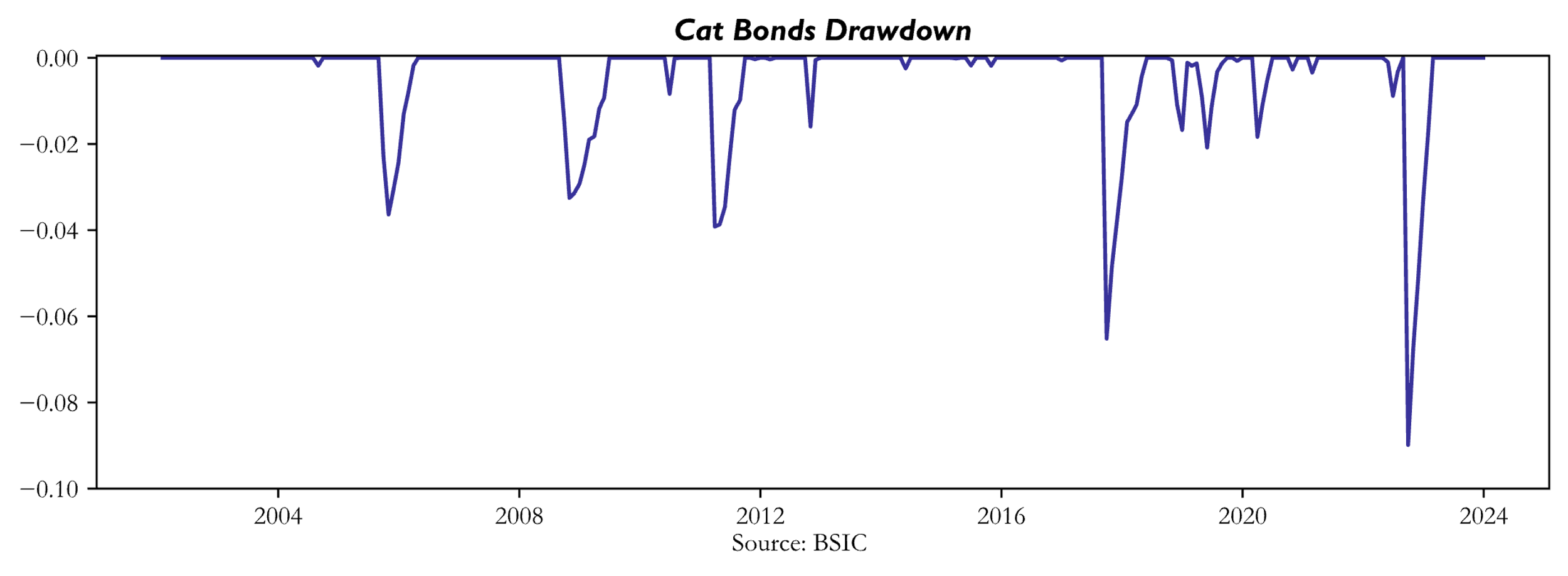
As seen from the previous chart, the index had consistent positive returns for every year in the sample excluding 2022. We now report the events that caused the main drawdowns in the index:

• 2005 Hurricane Katrina (August 23rd, 2005 – August 31st, 2005): yearly return for 2005 of +1.52%, worst month September 2005 with a return of -2.29%
• 2008 Impact by GFC: yearly return for 2008 of +2.27%, two consecutive months of negative returns September 2008 -1.49%, and October 2008 -1.79%. As Sterge and Van der Stichele (2016) report “cat bonds might not be diversifying in a liquidity crisis, even though such a crisis would have no effect on the likelihood or severity of events that would cause principal losses to the bonds themselves”.
• 2011 Great Tohoku Earthquake (March 11^th, 2011): yearly return of +3.33%, worst month March 2011: -3.92%
• 2017 Hurricanes Harvey (August 17^th – September 2^nd, 2017), Irma (August 30^th – September 12^th, 2017), and Maria (September 16^th – October 2^nd, 2017): yearly +0.46%, worst month September 2017: -6.52%
• 2020 Covid-19 (March 2020): yearly return of +5.82%, worst month March 2020 -1.84%. Similar reasons as the impact of the GFC in 2008.
• 2022 Hurricane Ian (September 23^rd September 30^th, 2022): yearly return -2.23%, worst month September 2023 with -8.99% loss.

Future Outlook

The CAT bonds market has seen substantial growth in recent years, particularly in 2023, which represented a record-breaking year in terms of issuances, for a total value of $16.5bn.

The main driver of CAT bond issuance is the frequency of natural catastrophes, that have a direct impact on the bonds default risk. Due to climate change, there is increasing uncertainty about weather patterns and the occurrence of said catastrophes, therefore leading to broader skepticism about the CAT bond market. Climate change’s impact cannot be overlooked: we are headed towards times where an increasing number of catastrophes needs to be considered. The effects on CAT bonds are double: we are likely to observe an increase in issuance and spreads, driven by the higher premium’s investors will demand for bearing the risk of an increasing number of catastrophes; however, for the same reasons, investors will be more hesitant to pour capital in the CAT bond market.

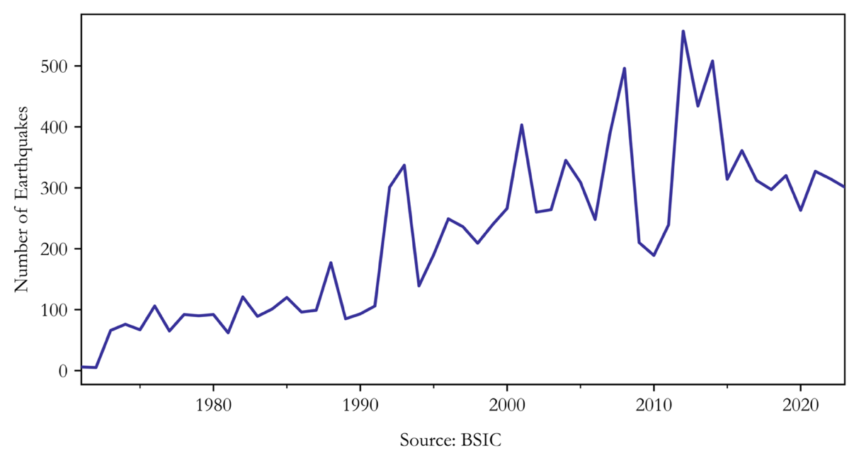
We must consider that climate change is a long-term phenomenon, and that CAT bonds typically have a short maturity: such a maturity is far too short to consider what might be the long-term effects of climate change. It is therefore more precise to observe specific climate trends and how they can influence the CAT bond market. There are a lot of observable patterns such as the El Niño Southern Oscillation (ENSO) or the North-Atlantic Oscillation (NAO). With regards to such patterns, we have tracked the frequency of earthquakes within 500km of the city of San Salvador and a clear trend emerges.

By analyzing smaller trends, we can better understand the direction in which CAT bonds are headed. Furthermore, given the number of CAT bonds available on the market for any specific region, research on local-related climate patterns is better to avoid drawing inaccurate conclusions.

In conclusion we believe that ultimately the high yields that the bonds offer will prevail, and the CAT bond market will continue to grow. The environmental impact of climate change will be accounted for in the bond’s pricing, which will reflect the higher default risk. However, CAT bonds have offered great diversification strategies to investors, given their little correlation to traditional financial markets and we believe that the specifics and variety of the bonds being issued will mitigate the risks of increasing natural disasters. For such reasons we think that the CAT bond market still has space to grow in the following years.

References

[1] Artemis, “Q4 2023 Catastrophe, Bond & ILS Market Report”, 2023.

[2] Difiore P. et al, “Catastrophe Bonds: Natural Diversification”, Neuberger Berman, 2021.

[3] Kousky C. and Braun A., “Catastrophe Bonds”, 2022.

[4] Lane, Morton N., “Rationale and results with the LFC cat bond pricing model”, 2003.

[5] Lee S. et al, “The world being on fire is swelling ‘catastrophe bonds’ to a record $45 billion—and it’s a key hedge fund strategy”,        Fortune.com, 2024.

[6] Motlagh F. et al, “Bonds for disaster resilience: A review of literature and practice”, International Journal of Disaster Risk Reduction, Volume 104, 2024.

[7] Siyamah I. et al, “Cat bond valuation using Monte Carlo and quasi Monte Carlo method”, 2020.

[8] Sterge A. and Van der Stichele B., “Understanding Cat Bonds”, The Journal of Alternative Investments, 2016.

[9] Swiss Re, “The Fundamentals of Insurance-Linked Securities.”, 2011.