Buy the Bubble Take the Ride

Introduction

“When I see a bubble forming, I rush in to buy, adding fuel to the fire.” This is a famous quote by George Soros. It probably inspired Jarrow and Kwok to write their paper, Inferring Financial Bubbles from Option Data where they attempt to take advantage of the theory of bubbles to create a profitable trading strategy. The theory behind it is fascinating. The real world, however, might disagree with it.

The Setting

We now introduce a model to detect financial bubbles using option price data rather than traditional time series price data. We refer to the paper “Inferring Financial Bubbles from Option Data” published in June 2021 by two professors Robert A. Jarrow and Simon S. Kwok. Specifically, they define an asset’s bubble associated with a selling time $t + \tau$ as the disparity between the market price and the fundamental value of the asset.

To obtain the fundamental price of the asset, we employ cross-sectional option price data to reveal the state-price distribution (SPD). The SPD represents the pricing mechanism of the underlying asset in the market. However, due to factors such as tail truncation and limited observation range beyond certain strike prices, the SPD lacks a parametric structure and cannot be entirely reconstructed.

As a result, the fundamental asset value and associated bubbles cannot be precisely pinpointed. Nonetheless, we try achieving partial identification of these values under certain mild restrictions. Two approaches are proposed for inferring asset price bubbles:

The first defines Naive Bound to infer the upper bound of the asset price bubbles. The second is a Simple Bounds Approach. This method establishes straightforward bounds based on options with extreme moneyness. The paper sets constraints on the potential range of asset price bubbles.

The simple bounds method acknowledges the possibility of put-call parity violations in market prices, indicating discrepancies between put and call option prices. By leveraging option price data and these proposed methodologies, it is possible to get insights into identifying and analyzing financial bubbles in asset markets.

Theory of bubbles

The theory behind our strategy and the paper itself is based on the recently developed local-martingale theory of bubbles. Given an Equivalent Local Martingale Measure (a probability measure such that each share price is exactly equal to the discounted expectation of the share price under this measure – it reflects the market pricing mechanism) according to the local-martingale theory of bubbles, a price process displays a bubble if it meets the criteria of being a strict local martingale under the ELMM. This means that the price process may exhibit characteristics of a martingale locally but deviates persistently from martingale behaviour over time.

A martingale is a sequence of random variables for which at a particular time, the conditional expectation of the next value in the sequence is equal to the present value, regardless of all prior values. A local martingale is a martingale in respect of the filtration of time. Local martingales play a crucial role in mathematical finance, particularly in the modeling of financial markets where phenomena like arbitrage and financial bubbles may lead to deviations from martingale behavior. These deviations are controlled by the stopping times $\tau_n$ , which indicates when to “stop” observing the process to ensure it remains a martingale. All martingales are local martingales however the converse is false and that is why there exists strict local martingales. While a local martingale may occasionally deviate from being a martingale within certain intervals, a strict local martingale exhibits this behavior persistently over time. A strict local martingale is not a martingale globally because it does not have zero expectation for all stopping times.

It has been shown (see Jarrow (2015)) that rational bubbles can exist with no-arbitrage and equilibrium. This allows the use of continuous time stochastic process mathematics to help estimate and test for the existence of asset price bubbles. With a stochastic process, a collection of random variables is indexed to some mathematical set called an index set. Each random variable in the collection takes a value from the state space with a certain probability. In a continuous stochastic process the index variable takes a continuous set of values.

By applying the concept of strict local martingales under an Equivalent Local Martingale Measure, the aim is to identify and analyze the presence of bubbles in financial markets. This approach provides a theoretical framework for understanding and characterizing the dynamics of asset price movements, particularly in scenarios where prices deviate significantly from their fundamental values.

The market settings are defined as follows. We start with a filtered complete probability space $(\Omega; \mathcal{F}; \mathbb{F}; \mathbb{P})$ where $\Omega$ is the state space representing all the possible outcomes, $\mathcal{F}$ is a $\sigma\$ , which is the information of the events up to time T, $\mathbb{F} = \{ \mathcal{F}_t \}_{0 \leq t \leq T}$ is the filtration of time and T is the terminal date which is assumed finite. The probability measure P, which assigns to each event in the space a probability, is the physical measure.

We assume the market is frictionless (no transaction cost and restrictions on trade), competitive (all investors are price-takers, no one has the market-share to influence the price on its own), and incomplete (there are more random sources than traded security). Market incompleteness is crucial so that bubbles can start, die, and be reborn within the model’s horizon.

For simplicity we suppose the market contains a money account and a single risky asset. Given $R_t$ and $S_t$ be respectively the value of a unit of money account and a unit of the risky asset at time t, we denote the time-t value of a unit share of each security as $U_t = (R_t, S_t)$ . The value of the portfolio at time t is $V_t = \eta_t R_t + \pi_t S_t$ .

The stochastic integral $(H \cdot U)_t$ represents the total profit generated by the portfolio generated by the trading strategy H over the period $[0, t]$ with the convention $(H \cdot U)_0 = 0$ . The trading strategy is considered to be F-admissible if it is self-financing, meaning it starts with zero initial investment and experiences no inflows or outflows over time, and if it does not lead to unbounded losses with positive probability.

Our strategy works under the assumption NFLVR (no free lunch with vanishing risk). It serves as a reinforcement of the non-arbitrage condition in a straightforward manner. According to the Fundamental Theorem of Asset Pricing, the No Free Lunch with Vanishing Risk (NFLVR) condition holds if and only if there exists a non-empty set $\mu_{\text{loc}}$ of equivalent local martingale measures (ELMM) under which the wealth process $V_0 + (H \cdot U)_t$ is a local martingale.

This condition enables the determination of the fundamental price of an asset, defined as the conditional expectation of the discounted cash flows of the risky asset, with the expectation taken under an ELMM. In an incomplete NFLVR market, there exists more than one such measure. The existence of this non-empty set is crucial as it permits the emergence, disappearance, and resurgence of an asset price bubble.

All assets (both the money account and the risky asset) are undominated on (0, T]. Let recall that an asset A is undominated if there is not another asset B such that under “any” realizations of the financial future asset B will provide a “larger total return” than asset A.

We also assume continuous trading over a finite horizon and explore a specific type of bubble that can arise in this setting only. This bubble phenomenon pertains to an asset whose risk-adjusted expected discounted cash flows, upon liquidation at any finite time, is lower than the market price. Consequently, the asset’s price process is characterized as a local martingale but not a martingale, consistent with the local-martingale theory of bubbles.

Now suppose the market selects the ELMM $Q_t \in \mu_{\text{loc}}$ at time t. Under this probability measure the fundamental price of the risky asset is defined as the expected, risk adjusted and discounted cash flow we get at the liquidation of the asset at the model’s horizon T.

However, when dealing with options, a generalization of this definition is necessary because the fundamental value of an option depends on the market price of the underlying asset on the option’s maturity date, which typically precedes T. So we need to define the time-t fundamental price of the risky asset to be sold at time $t + \tau$ where $\tau \leq (T - t)$ . That is:

$\mu_{t}^{*} = \mathbb{E}_{t}^{*}[R_{t}^{-1}R_{t + \tau} S_{t + \tau} ]$

The associated bubble of the risky asset with selling time $t + \tau$ is defined as the difference between the market and fundamental prices of the asset:

$\Pi_{t}^{S}(\tau) = S_{t} - \mu_{t}^{*}$

This bubble estimate varies depending on the selling date of the asset, reflecting the declining expectation as the time to the asset’s selling date decreases.

Now let $C_t(k, \tau)$ and $P_t(k, \tau)$ be the t-time market prices of the European call and put options written on the risky asset with strike price k and time-to-maturity $t + \tau$ where $\tau \leq (T - t)$ . Under ELMM their time-t fundamental prices are defined to be:

$C_t^*(k, \tau) = \mathbb{E}_t^*[R_{t}^{-1}R_{t + \tau}(S_{t + \tau} - k) _+]$

$P_t^*(k, \tau) = \mathbb{E}_t^*[R_{t}^{-1}R_{t + \tau}(k - S_{t + \tau}) _+]$

We define options’ bubbles as the difference between their market and fundamental prices:

$\Pi_{t}^{C}(k, \tau) = C_t(k, \tau) - C_t^*(k, \tau)$

$\Pi_{t}^{P}(k, \tau) = P_t(k, \tau) - P_t^*(k, \tau)$

These expressions capture the deviation of option market prices from their corresponding fundamental values, reflecting market inefficiencies or speculative activity.

Under assumption NFLVR we can prove that, $\Pi_{t}^{S}(\tau) \geq 0, \Pi_{t}^{C}(k, \tau) \geq 0$ and $\Pi_{t}^{P}(k, \tau) \equiv 0$ . In simpler terms, a bubble arises when people buy an asset with the expectation of selling it in the future at a higher price. However, if there’s a limit to how high the price can go, such as with put options, then this expectation becomes unrealistic, and bubbles cannot occur. So assets whose price is bounded above can have no bubble, that is the case for put options.

In practice, during crises or periods of market panic, there might be a rush to buy put options with lower strike prices, reflecting a desire to protect against further losses. This increased demand for these options can impact their market prices, potentially lowering them. As a result, the estimated fundamental price of the underlying asset (determined by factors like the probability distribution under the Equivalent Local Martingale Measure) might decrease as well, particularly if there’s a higher likelihood of extreme negative events. However, the previous statement suggests that despite changes in the fundamental value of the asset due to panic sales, the market price of put options remains aligned with their fundamental value under the principle of no-arbitrage. This means that even though panic selling may affect perceptions of the asset’s value, the market price of put options should still accurately reflect their intrinsic worth, given prevailing market conditions and risk factors.

We also assume for call options a bubble independence from strike prices. This implies that the market prices of calls satisfy $C_t(k_1, \tau) > C_t(k_2, \tau)$ if $k_1 < k_2$ . This condition is likely to hold in option markets because its violation would immediately invoke market transactions.

Indeed, it’s highly unlikely to observe two call options, let’s say A and B, where the strike price of A is greater than the strike price of B, yet the price of A is less than the price of B. Such a scenario would likely prompt market participants to exploit the arbitrage opportunity, leading to adjustments in prices to restore the expected relationship between call option prices and strike prices.

Identifying the SPD and Fundamental price from Option Data

Let consider a scenario where a share of the risky asset is priced at $S_t$ at time t. At this moment, the market selects an Equivalent Local Martingale Measure (ELMM) denoted as $Q_t^*$ . We’ll use the same notation $Q_t^*$ to refer to the cumulative distribution function of $S_{t + \tau}$ given $\mathcal{F}_t$ , where $\tau$ represents a fixed holding period. $Q_t^*$ represent the state price at $t + \tau$ given $\mathcal{F}_t$ , that is the conditional state price distribution given by: $Q_t^* = \{S_{t + \tau} \leq s\} = Q^* \{S_{t + \tau} \leq s \| \ \mathcal{F}_{t}\}$ . We can assume a constant risk-free spot interest rate r, which implies that $R_t = e^{rt}$ . This simplifies the calculation of discount factors and expected values under the ELMM.

We can compute the fundamental price of the asset in the following way, if $Q^*$ is precisely known:

$\mu^* = \int_{0}^{\infty} e^{-r\tau}sdQ^* (s) \ = \int_{0}^{\infty} e^{-r\tau} [1 - Q^* (s)]ds$

The formula used for the computation parallels the one used to infer time-t fundamental price of the risky asset to be sold at time $t + \tau$ , described previously. However since $Q^*$ is not revealed beyond the strike price range, we cannot evaluate exactly the value of $\mu^*$ using this formula. Nevertheless, we can obtain reasonable bounds on the contribution from the truncated tails of $Q^*$ .

For finite $l, u > 0$ , we have:

$\int_{0}^{l} e^{-r\tau} [1 - Q^* (s)]ds \ = e^{-r\tau}l - P^* (l)$

$\int_{u}^{\infty} e^{-r\tau} [1 - Q^*ds] \ = C^* (u)$

Note that we consider $C^*(\infty) = 0$ . Now let $u = u_c$ be the maximum strike for calls and $l = l_p$ the minimum strike for puts. Let decompose the integral above as follows:

$\int_{l_p}^{u_c} e^{-r\tau} [1 - Q^* (s)]ds \ + [e^{-r\tau}l_p + C^* (u_c) - P^* (l_p)]$ .

Now the integral is over the available range of strike prices and this means we can actually evaluate it. The other term of the formula represents the contribution from the two tails of $Q^*$ . In the formula are included the fundamental values of the put and call options, which are unobserved but can be bounded as follows:

$-P(l_p) \leq C^*(u_c) - P^*(l_p) \leq C(u_c)$

These deducted bounds provide us with a very narrow range. Indeed $C(u_c)$ and $P(l_p)$ denote the prices of the most out-of-the-money calls and puts which are also the least expensive options available on the market.

Naive Bounds and Simple bounds on Asset Price Bubbles

This method represents the first of two approaches utilized to infer asset price bubbles, as introduced earlier. It constructs simple bounds on asset price bubbles by aggregating calls and putting price data whenever feasible. Specifically, it involves considering the prices of options with extreme moneyness.

Let $[l_c, u_c]$ and $[l_p, u_p]$ denote the range of strike prices for calls and puts and consider all the six combinations of these ranges. Given that, we can construct under NFLVR assumption and call option’s bubble k-independence, the following bounds on asset price bubbles.

$L_1 = S_t - e^{-r\tau}l_c +P(l_c) - P(l_p) - C(l_c), \quad U_1 = S - e^{r\tau}l_c + P(l_c) + C(u_c) - C(l_c),$

$L_2 = S - e^{-r\tau} u_p + P(u_p) - P(l_p) - C(u_p), \quad U_2 = S - e^{r\tau}u_p + P(u_p) + C(u_c) - C(u_p),$

$L_3 = S - e^{-r\tau}l_p - C(l_p), \quad U_3 = S - e^{r\tau}l_p + P(l_p) + C(u_c) - C(l_p),$

$L_4 = S - e^{r\tau}u_c + P(u_c) - P(l_p) - C(u_c), \quad U_4 = S - e^{r\tau}u_c + P(u_c),$

$L_5 = S - e^{-r\tau}l_c + P(u_p) - P(l_p) - C(l_c), \quad U_5 = S - e^{r\tau}u_p + P(u_p) + C(u_c) - C(l_c),$

$L_6 = S - e^{-r\tau}l_p - C(u_c), \quad U_6 = S - e^{r\tau}u_c + P(l_p).$

and for fixed time t and for any time to maturity $\tau$ , and for any $\omega \in [0, 1]$ we have:

$(a) \quad \max \{0, \omega L_1 + (1-\omega) L_2\} \leq \Pi^{S} \leq \omega U_1 + (1-\omega) U_2 \quad \text{for} \ l_p \leq l_c < u_p \leq u_c$

$(b) \quad \max\{0, \omega L_3 + (1 - \omega)L_4\} \leq \Pi^{S} \leq \omega U_3 + (1 - \omega) U_4 \quad \text{for} \ l_c \leq l_p < u_c \leq u_p$

$(c) \quad \max \{0, \omega L_1 + (1 - \omega) L_4\} \leq \Pi^{S} \leq \omega U_1 + (1 - \omega) U_4 \quad \text{for} \ l_p \leq l_c < u_c \leq u_p$

$(d) \quad \max\{0,\omega L_3 + (1 - \omega)L_2\} \leq \Pi^{S} \leq \omega U_3 + (1-\omega)U_2 \quad \text{for}\ l_c \leq l_p < u_p \leq u_c$

$(e) \quad \max\{0, L_5\} \leq \Pi^{S} \leq U_5 \quad \text{for} \ l_p < u_p < l_c < u_c$

$(f) \quad \max\{0, L_6\} \leq \Pi^{S} \leq U_6 \quad \text{for}\ l_c < u_c < l_p < u_p$

These simple bounds are derived to estimate asset price bubbles by decomposing the integral from the previous section into different intervals defined by the ordinal measure assigned to the values of $l_c, l_p, u_c, u_p$ and repeatedly applying the computation explained above. Wherever the strike ranges overlap the bounds may be expressed in terms of the call or put prices, or as a linear combination of them (the weight $\omega \in [0, 1]$ indicates the proportion of the bound expression contributed from calls).

The width of the interval obtained from this computation represents the degree of uncertainty we have on inferring the exact value of the asset price bubble. This uncertainty arises because information about $Q^*$ is not fully recovered beyond the bounded range of strike prices.

If we then apply both NFLVR and non-dominance assumptions we get the following result as a naive bound for asset price bubbles:

$0 \leq \Pi^{S} (\tau) \leq C(u_c, \tau)$

Intuitively, under non-dominance the asset price bubble is equal to the call bubble, which is bounded above from the call price. We can prove that also by observing that under these conditions, put-call parity in market prices hold and the inequalities (a) and (d) reduce to the stated bound.

Strategy

We now try to apply the theory above by using the estimated bubbles to construct a profitable momentum trading strategy following the one presented in the paper and extending it to other indices besides the S&P 500 (Nasdaq 100, Dow Jones, Russel 2000).

We collect daily prices of European call and put options written on the indices between 1999 and 2024 from OptionMetrics. Data are filtered by retaining only options with positive traded volume, price above $0.05 and expiry date before the 27Th of a month to remove all “non-standard” contracts. Additionally, we filtered by time to maturity, considering only options expiring between 8 and 90 days as this range is the most traded one.

From option prices we computed both the Naïve bounds and Simple bounds but, given that the former assume the put-call-parity is valid, while this does not empirically hold in the market, we decided to use Simple bounds when implementing the strategy. These are computed by using formula (a) reported above, whose validity condition actually holds in the data.

We implement a joint momentum strategy based on the index level (S) and its bubble estimate ( ${\hat {\Pi}}^S$ ). The idea is to take a long position when either the bubble estimate or the index exhibits an upward trajectory and to deposit the proceeds into a money account with zero interest when not holding the index. Particularly, let $MA_{i}(S)$ and $MA_{i}({\hat {\Pi}}^{s}(\tau))$ be, respectively, the ith moving averages of S and ${\hat {\Pi}}^S$ over a rolling window of 3 months for i=1 and 1 year for i=2. The strategy suggests holding the index at time t if:

$MA_{1}({\hat {\Pi}}^{s}(\tau))_t > MA_{2}({\hat {\Pi}}^{s}(\tau))_t \quad or \quad MA_{1}(S)_{t} > MA_{2}(S)_{t}.$

To hold while the bubble is expanding may be counterintuitive, but such a strategy is motivated by the “greater fool” theory regarding the formation of bubbles. According to this theory, investors can profit from buying overvalued assets with the expectation of selling them later to a “greater fool” at an even higher price, regardless of the underlying fundamentals of the asset. This of course is risky, because it relies on the continuous availability of buyers willing to pay higher prices. The strategy aims to surf the bubble while expanding and selling before it bursts.

By construction, the strategy is a more aggressive version of the pure momentum strategy. To better analyze the results, we compare these two strategies with the buy and hold one.

Results

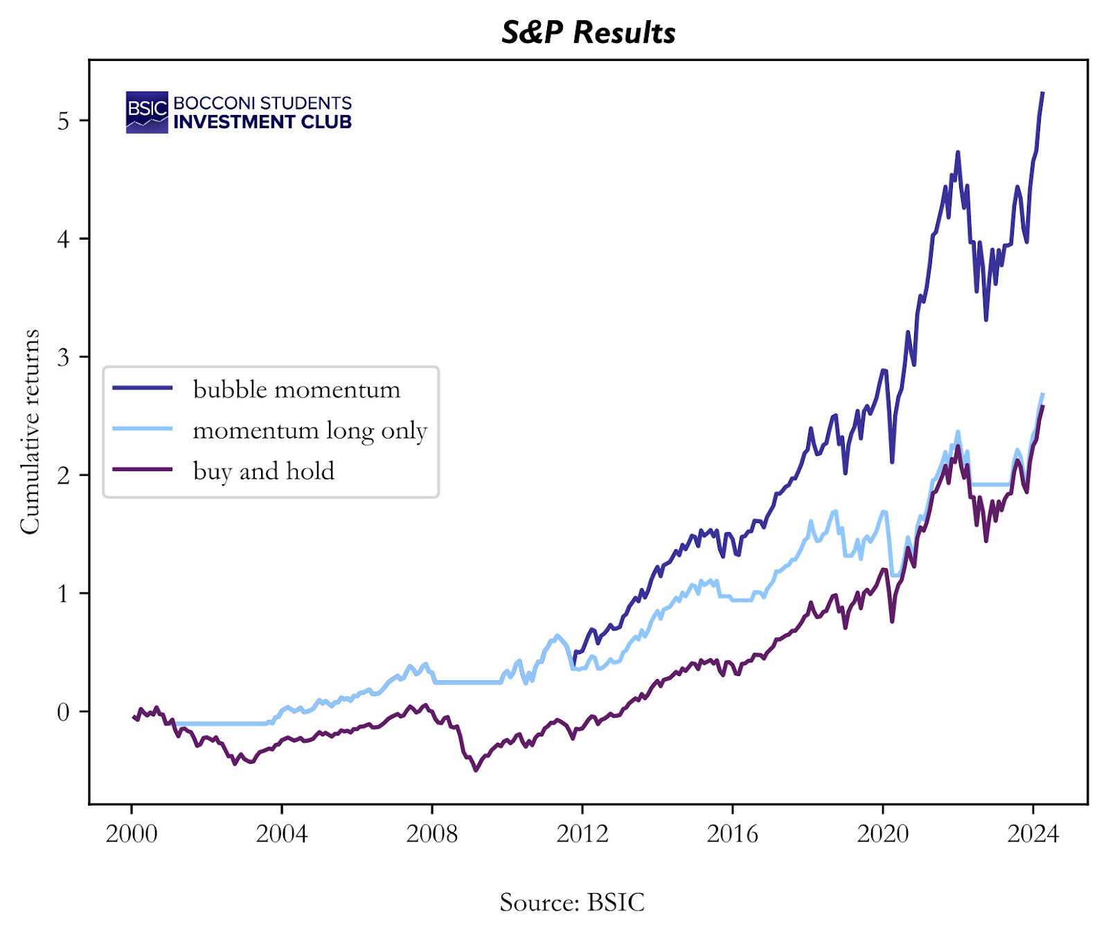
After recreating the simple bounds and running the strategy as explained above, we managed to get similar results for the S&P 500 index. We observe that the bubble momentum strategy achieves worse returns compared to buy&hold and long-only momentum between 1999 and 2024.

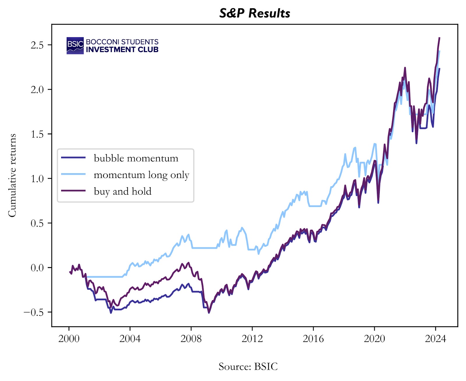
A graph showing the growth of the stock market Description automatically generated

That is a red flag since in the paper the strategy outperformed the buy and hold by a wide margin. There is a small difference that our data set begins four years later than theirs but ends 9 years later. So, our data set is larger. This difference should not account for the difference in performance if the strategy were robust enough. That’s why we decided to look at the performance of the strategy for some other indexes, namely, Nasdaq-100, Russel-2000, and the Dow.

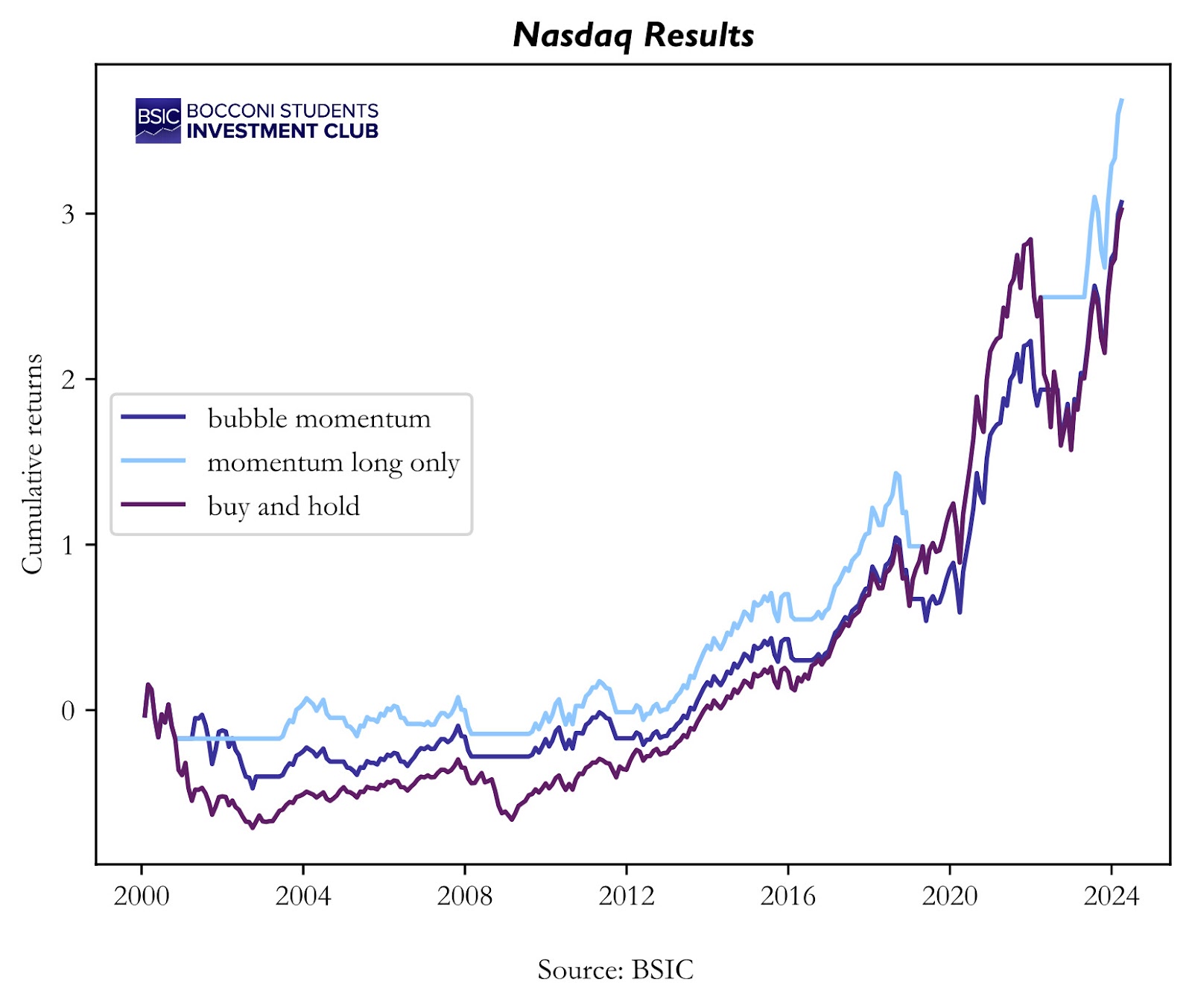
A graph showing the growth of the stock market Description automatically generated

Here is our first sign that something isn’t working. The strategy performs worse than the buy & hold for the NASDAQ-100 as well. Anyways, maybe the NASDAQ was another exception, and the strategy performs incredibly well for other indexes. Let’s try the Russell 2000

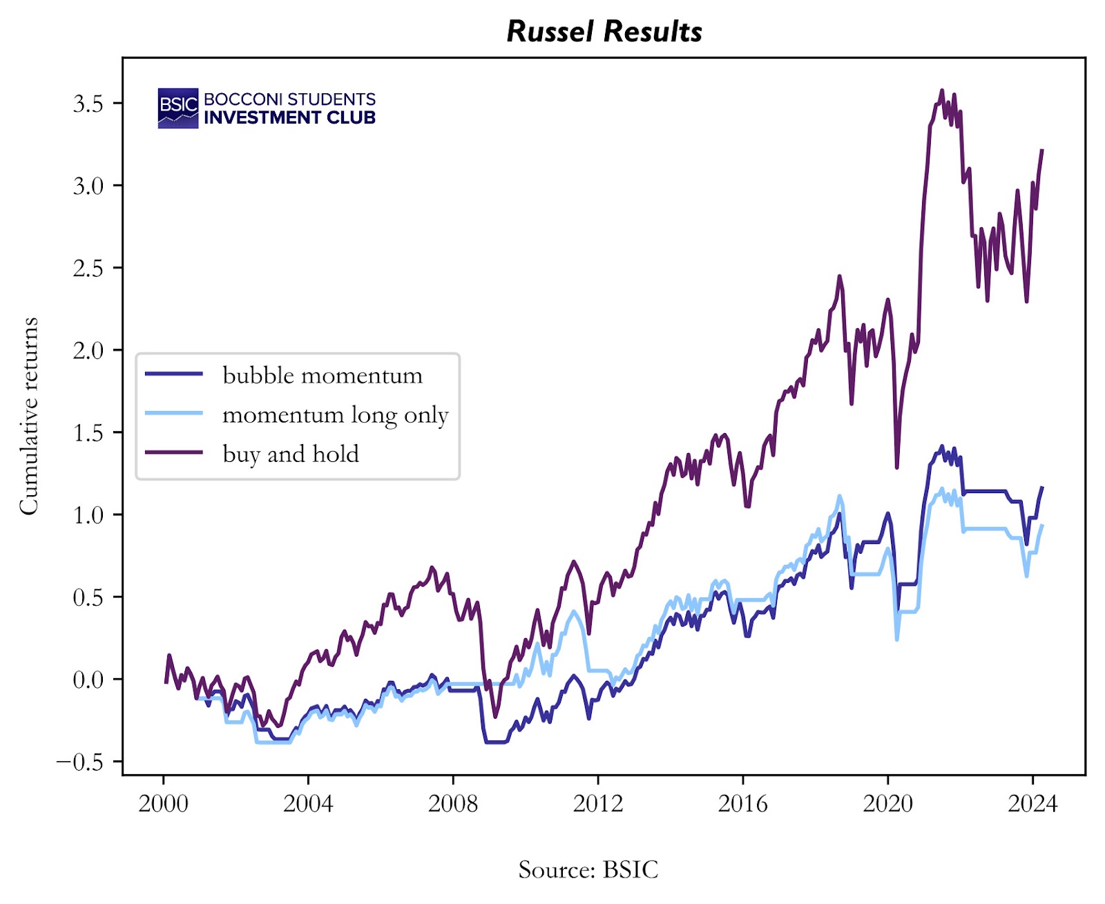
A graph showing the results of a stock market Description automatically generated

Nope. Our strategy underperforms the buy & hold again. Maybe this time it is because we are out of the market for longer. To determine what is true, we are going to look at the annualized average returns for each strategy.

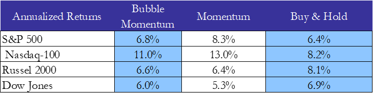
A screenshot of a graph Description automatically generated

Source: BSIC

Here we can finally see that in fact, the strategy does have higher returns when we look at the NASDAQ-100 and S&P 500. So 2 points go to the bubble strategy? Not really because when we add the Dow we see that the strategy has less returns than the buy & hold for that as well. Not to mention that the momentum strategy outperform the bubble strategy both for the Nasdaq-100 and the S&P 500

This is getting a bit frustrating. The strategy seems to be working, although inconsistently. Also, these are US equity indices and our strategy is long only, so it is expected that it’s going to make money, the problem is that for some indices it underperforms and for others it outperforms.

Maybe the secret is hidden in the Sharpes of the strategies.

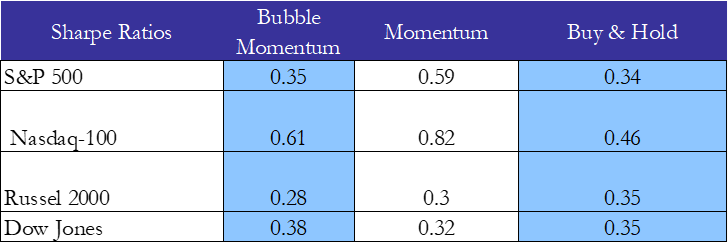
A screenshot of a graph Description automatically generated

Source: BSIC

Maybe not. We can see that indeed for some indices the strategy improves the Sharpe, but not as much as the Momentum. For others both momentum and bubble momentum underperform. So even though there is some evidence to support the validity of that strategy it is not nearly enough.

We found it peculiar that the authors of the paper use a moving average cross to define momentum since we usually see it defined as just past performance predicting future returns.

That is why we propose our own version of the strategy: instead of verifying when the three-month moving average crosses the yearly moving average, we rely only on the latter, holding the indices when it increases either for the index value or bubble estimation. This allows the strategy to be more reactive when the market crashes.

Thus, we hold the index at time t if:

$MA({\hat {\Pi}}^{s}(\tau))_t > MA({\hat {\Pi}}^{s}(\tau))_t-1 \quad or \quad MA(S)_{t} > MA(S)_{t-1}.$

For our version, we get a much better performance on the S&P, with a better Sharpe as well.

A graph showing the growth of the stock market Description automatically generated

However, if we are being honest, our strategy still struggles to beat pure momentum in terms of Sharpe.

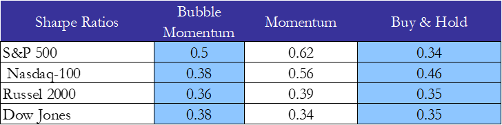
A screenshot of a graph Description automatically generated

Source: BSIC

Here we can see that the strategy applied to the S&P 500 destroys the buy & hold in terms of Sharpe (and in terms of returns to be honest), but that’s about it. For all the rest it performs worse or similarly. Compare that with the momentum strategy, which is taking advantage of a long established risk factor. Momentum has a better Sharpe for almost all indices except the Dow, but even for the Dow, it is only 0.01 points lower. All of this leads us to believe that this strategy is not robust at best. We did not feel the need to test the statistical significance of those results since they were inconsistent enough as it is.

A screenshot of a graph Description automatically generated

Source: BSIC

As you can see, the annualized results of the strategy are even more inconsistent than the Sharpe. All in all, we will recommend just investing in the index if you care about returns, and using momentum if you care about the Sharpe.

Conclusion

We have a small concession to make. The strategy that we tested is a simpler version of the one used in the paper. While this might detract from our case, the point still stands. The authors should have tested the strategy on other instruments, not just the S&P 500. That would also include non-equity indices as well because equities tend to move up with time and long-only strategies will consequently tend to make money as long as they are not horrendously and managed to time the market so poorly that they lost money over 20 years.

There are some improvements to be made as well. One we already mentioned. We could also backtest the exact strategy that was used in the paper and check if that would substantially change the results, although we are doubtful about that. Something else that we could improve on is the strategy itself since buying when the bubble is inflating seems a bit simplistic and dangerous.

References:

[1] Jarrow, Robert A., and Simon S. Kwok. “Inferring Financial Bubbles from Option Data”. Journal of Applied Econometrics, vol. 36, no. 7, Nov. 2021, pp. 1013-46. DOI.org (Crossref), https://doi.org/10.1002/jae.2862.

Published by BSIC on 31 March 202431 March 2024

0 Comments

Leave a Reply Cancel reply

Corporate Finance Markets

Exploring the Practicality of Merger Arbitragе

Markets

Market Recap 05/05/2024

Markets

A Systematic Approach to Credit Investing

Buy the Bubble Take the Ride

Published by BSIC on 31 March 202431 March 2024

0 Comments

Leave a Reply Cancel reply

Related Posts

Corporate Finance Markets

Exploring the Practicality of Merger Arbitragе

Markets

Market Recap 05/05/2024

Markets

A Systematic Approach to Credit Investing