Feature Selection and Engineering for Time Series Data

Download PDF

Introduction

Feature engineering and selection are crucial for optimizing machine learning models. Through thoughtful feature engineering, models can capture essential insights from the data, which may otherwise remain hidden, thereby improving the predictive accuracy. On the other hand, effective feature selection reduces model complexity, which not only speeds up the training process but also minimizes the risk of overfitting. This leads to more robust, generalizable models that perform well on unseen data. Together, these processes significantly enhance the overall utility and effectiveness of machine learning applications, making them indispensable in the field.

Feature Selection

Feature selection is the process of identifying the optimal subset of features that contributes to the predictive power of a model, based on various criteria. These criteria include enhancing the interpretability of the model’s results—since a model with fewer features, such as 5 instead of 100, is typically easier to understand. It also involves reducing the complexity of the algorithm, which often scales with the number of features (), helping to prevent issues like overfitting. This is particularly relevant in models such as Linear Regression, where linear dependence among features can lead to overfitting. Additionally, feature selection can decrease the model’s loss, which may be exacerbated by noisy data in the features. Each of these reasons can be crucial depending on the specific context of the analysis.

There are three main methods of feature selection: filter methods, wrapper methods, and embedded methods. We will explore each of these in further detail.

Filter methods

Filter methods assess the relevance of features based on statistical measures, independent of any specific machine learning model you might plan to use. When dealing with features that are discrete, various statistical methods can be applied to evaluate their usefulness.

A key concept in understanding filter methods is entropy, denoted as . It is calculated using the formula:

This measure quantifies the uncertainty in a system. Entropy reaches its maximum when the probabilities of different outcomes are equal, indicating high uncertainty or randomness in the outcome. For instance, consider a fair coin with two outcomes where each has a probability of 1/2; in this case, you gain no additional information from the outcome because it is entirely random, hence entropy is at its maximum (. Conversely, if a coin has heads on both sides, there is no uncertainty since the outcome is always the same, resulting in an entropy of . Therefore, the lower the conditional entropy , the more information a feature provides, as it reduces uncertainty about the outcome Y.

Information Gain (IG)

IG quantifies how much knowing one variable, X, helps in predicting another variable, Y. It is calculated as:

This measures the reduction in entropy from knowing X about Y. Information Gain is zero when X and Y are independent, meaning that knowledge of X provides no information about Y. It reaches its maximum value when X completely determines Y, thus completely reducing the uncertainty about Y.

The Chi-squared test

The Chi-squared test is a statistical method used to determine if there is a significant difference between expected and observed data. It is given by the formula:

Let’s review a simple binary example where both X and Y

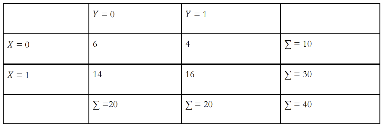
Under the assumption of independence between X and Y, the expected count for the case where both X and Y are zero would be calculated as follows: , but in observed data it is 6, so the contribution to the Chi-squared statistic for this cell is: . To assess whether the observed deviations from expected frequencies are significant, one would compare the calculated Chi-squared statistic to the critical values from the Chi-squared distribution with degrees of freedom calculated as . In this case, with a 2×2 table, there is 1 degree of freedom.

The concept of degrees of freedom typically involves subtracting one because it accounts for the constraints already known about the data. For instance, if you know the total sum of two variables, knowing one value automatically fixes the other. This constraint reduces the number of independent values that can vary, which is why we subtract one.

Handling Low Variance Features

Low variance features in a dataset often indicate that a variable does not vary much between observations. Typically, a feature with minimal or no variation might be considered for removal because it contributes little to no additional information to a model and could potentially introduce unnecessary noise. However, it’s crucial to approach the removal of such features cautiously. Even though a feature may exhibit low variance, it could still hold valuable information under certain conditions. For instance, a feature that mostly assumes a constant value but changes under specific circumstances could be highly informative about those conditions. Therefore, the decision to remove a low variance feature should be well-considered, weighing the potential loss of subtle but important data against the simplicity and efficiency gained by its exclusion.

Utilizing ANOVA F-Test for Feature Selection

The Analysis of Variance (ANOVA) F-test is a statistical method used to compare the means of three or more groups to determine if at least one of the group means significantly differs from the others. It extends the principles of a t-test to more than two groups, making it ideal for testing the differences between the means of several independent (unrelated) groups.

The formula for the ANOVA F-test statistic is:

Here, k represents the number of groups, is the number of observations in each group, is the overall mean of all observations,​ is the mean of group i, and N is the total number of observations.

While the statistic itself may seem complex, its practical application is straightforward. For instance, consider a dataset containing various features of cars, where you are interested in predicting car prices. If an ANOVA test is performed between the car brand (a categorical feature) and car prices, and it reveals significant differences in mean prices across different brands, this indicates that car brand significantly influences car prices. Thus, this result would suggest that including the car brand feature in a predictive model for car prices is crucial.

In summary, the ANOVA F-test in feature selection helps identify categorical features that significantly segregate your continuous outcome variable into groups with distinct means. This indicates these features are significant predictors of the outcome, aiding in more accurate and effective model building.

Understanding Correlation in Feature Selection

Correlation between features plays a crucial role in selecting the right variables for a predictive model. If a feature shows a strong correlation with the target variable, it is likely a valuable predictor and should be retained. Conversely, if two features are highly correlated with each other, it might be beneficial to remove one to avoid redundancy. This process helps in simplifying the model without losing significant predictive power.

In different scenarios, different types of correlation coefficients can be utilized to measure relationships:

• Pearson’s Correlation Coefficient: This is used to assess the linear dependence between variables. It’s ideal for situations where the relationship between variables is expected to be linear.
• Spearman’s Correlation Coefficient: This measure is used for estimating monotonic relationships, regardless of whether they are linear. This is useful when the relationship might not be linear but consistently increases or decreases.
• Kendall’s Rank Correlation Coefficient: This is particularly effective for assessing the ordinal relationship between two variables and is robust against outliers or non-linear relationships.

These concepts extend to time series data, where dependencies between time steps can be analysed using the Autocorrelation Function (ACF) or Partial Autocorrelation Function (PACF). ACF helps identify the correlation of a series with its own lagged values, while PACF measures the correlation of the series with its lagged values, discounting the contributions from the intervening comparisons. These tools are instrumental in identifying patterns within time series data that are predictive of future values.

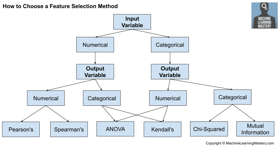
Source: How to Choose a Feature Selection Method For Machine Learning by Jason Brownley.

Filter methods serve as a fundamental approach to feature selection, providing a quick and straightforward means to assess the importance of individual features without considering the model that will eventually be used. These methods rely on various statistical measures to determine the relevance of each feature to the target variable. While effective, it’s important to remember that filter methods evaluate each feature in isolation, which may not always capture the full context in which the features operate together.

A common scenario where filter methods can be misleading is when examining features one at a time. For instance, when projecting data on individual axes, the distribution of classes might appear random and thus suggest no significant relationship between the features and the target. However, if the same data is viewed in a multidimensional space (such as a 2-dimensional plot), clear patterns and relationships can emerge, demonstrating interactions between features that are not apparent when viewed separately.

Most of the techniques used in filter methods, including various forms of correlation and statistical tests like ANOVA and Chi-squared, are well-integrated into libraries such as sklearn. This integration simplifies the practical application of these methods in feature selection processes.

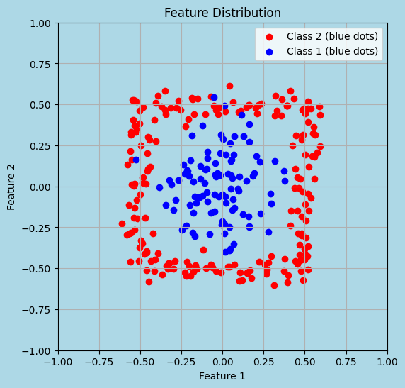
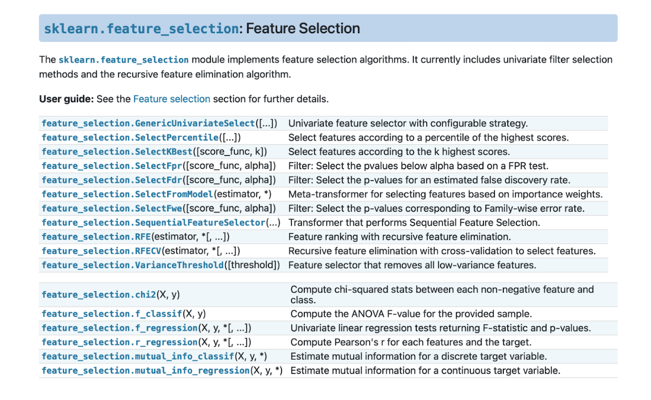
Source: Sklearn API

Wrapper Methods

Wrapper methods involve a more targeted approach to feature selection compared to filter methods. They directly integrate the model performance as a criterion for evaluating different subsets of features. This method involves sampling various combinations of features, applying a specific machine learning algorithm to these subsets, and then selecting the subset that delivers the best performance results.

Different Techniques Within Wrapper Methods:

• Backward Stepwise Selection: This technique starts with all available features. Iteratively, it removes the least significant feature (the one whose absence least affects the model performance) until a predetermined stopping criterion is reached, typically a desired number of features or a performance threshold.
• Forward Stepwise Selection: In contrast to the backward approach, this method begins with no features and adds the most significant feature at each step. This process continues until adding new features no longer offers a substantial improvement in the model’s performance.
• ADD-DEL Feature Selection: This method combines elements of both forward and backward selection. It alternates between adding and removing features to refine the feature set dynamically. This approach allows for flexibility in exploring the feature space more extensively.
• Subset Selection: This technique tests the model on various subsets of features up to a certain size. While theoretically, the best subset could be determined by exhaustively comparing all possible combinations, this approach becomes computationally expensive as the number of features grows, with complexity increasing exponentially.

Optimization Techniques in Subset Selection:

Given the potentially prohibitive computational cost of exhaustive search in subset selection, alternative strategies are employed:

• Directional Search: This optimization technique aims to find a local optimum by exploring the neighbourhood of the current feature set. It systematically tests slight variations of the current subset to see if performance can be incrementally improved.
• Stochastic Methods: These methods, including genetic algorithms, offer a way to navigate the search space more randomly yet effectively. Genetic algorithms, for example, use mechanisms inspired by biological evolution, such as mutation, crossover, and selection, to explore and optimize feature combinations.

While wrapper methods can provide a highly effective means to determine the optimal feature set for a specific model, their computational intensity and dependence on the chosen model make them less scalable for very large datasets or feature sets. Nevertheless, their ability to tailor feature selection closely to the performance of the model often results in more predictive and efficient models when computational resources allow.

Source:  From Linear Regression to Ridge Regression, the Lasso, and the Elastic Net, Robby Sneiderman

Embedded methods 

Embedded methods are a class of feature selection techniques that are directly incorporated into the training process of specific machine learning models. These methods are inherently efficient as they optimize model performance and complexity simultaneously by selecting relevant features during the model training phase.

In models like linear regression, the significance of features can often be inferred from the weights or coefficients assigned to them. Larger absolute values of coefficients indicate a stronger influence on the model’s predictions. However, it’s essential to scale your data before training to ensure these weights accurately reflect the importance of features, as unnormalized data can distort these values.

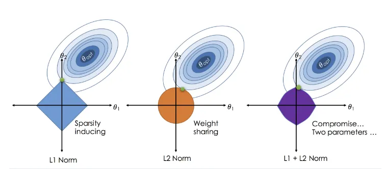
LASSO Regression is an embedded method particularly well-suited for scenarios involving numerous features. The effect of LASSO can be visually understood through its geometric properties, especially in cases with two features, where the LASSO constraint—shaped like a diamond—often intersects optimization contours at axes, leading to the elimination of some variables.

Decision tree algorithms, including their ensemble versions like random forests and gradient boosting machines, also inherently perform feature selection. They do this by choosing the best features for splitting nodes, thus incrementally building an efficient and effective model. The importance of each feature in these models is typically assessed based on how much it reduces the impurity of the nodes. However, these tree-based methods can sometimes show a preference for features with a larger number of unique values or categories, potentially skewing the importance metrics.

To address biases in tree-based methods, permutation feature importance is often used. This method involves randomly shuffling the values of each feature and measuring the resultant drop in model performance. A significant decrease in performance indicates a high dependency on the shuffled feature, thus providing a more accurate measure of its significance.

Principal Feature Analysis (PFA)

Most of the readers might be familiar with the PCA method that helps reduce the dimensionality of the feature space. However, the problem with PCA is that strictly speaking it is not a feature selection method as it does not preserve the original features but rather creates new ones that are linear combinations of the existing ones. The PFA method battles this problem with trying to select a subset of features from the original feature space. PFA uses the structure of the principal components to identify groups of features that capture the most variance. By clustering the rows of the matrix of principal components and then selecting representative features from these clusters, PFA maintains the physical interpretation of the original variables. The selected features are those that contribute most to each principal component, preserving the meaning and interpretability of the original data.

The authors describe the PFA process in five steps^[1]:

1. Compute the covariance (or correlation) matrix.
2. Perform PCA to get principal components and eigenvalues.
3. Decide on the subspace dimension q to retain a certain amount of data variability.
4. Use clustering (K-Means) on the rows of the principal components to find groups of correlated features.
5. Choose the central feature from each cluster to represent that group optimally.

However, if you do not have the necessity to preserve the original feature space, it is important to understand that PCA is usually used on stationary data and can lead to incorrect inferences. We will deal with stationarity later in the article, but those who are interested in the topic we suggest take a look at a recent paper by one of the leading innovators in the field of econometrics of the past years James D. Hamilton who together with Jin XI develops a new method for applying PCA to a mix of stationary and nonstationary variables without needing to first determine which variables are which^[2].

Feature Engineering

Feature engineering is the transformation of raw data into meaningful features in order to improve the performance of predictive models. It involves creating and transforming features to accurately capture underlying patterns and relationships.

The temporal indexing of time series data brings unique complexities that require specialized techniques to extract relevant features that effectively capture temporal patterns, trends and seasonality. Through feature engineering, one aims to improve model performance, interpretability, and forecasts in time series analysis.

Particularly, financial time series are usually non-stationarity, while to perform inferential analysis it is necessary to work with invariant processes, thus, it is common to transform data to make the series stationary.

Stationarity

In the context of time series analysis, stationarity refers to a property of a stochastic process where the statistical properties of the data remain constant over time. By definition a stochastic process {y_t} is said to be (covariance) stationary if it has time invariant first and second moments, i.e., if for any choice of t=1,2,…, the following conditions hold:

Thus, a stationary time series is characterized by a constant mean, constant variance, and constant autocorrelation at all lags, meaning that the overall structure of the data remains consistent over time, without any systematic trends, seasonality, or other patterns that evolve or change with time.

The simplest example of a stationary process is the White Noise, which is defined as a sequence of random variables with mean equal to zero, constant variance equal to and zero autocovariances except at lag zero. The White Noise can be seen as the fundamental building block of all stationary processes, in fact, following Wold’s Decomposition Theorem, every (covariance) stationary, non-deterministic, stochastic process can be written as an infinite, linear combination of white noise components.

On the other hand, a random walk is an example of a non-stationary time series as its variance changes over time. In fact, supposing to be a random walk process, and thus , where is a random error term with mean zero and variance , it is easy to compute that , and .

Removing trends

In finance time series are often non-stationary and this may be linked to the presence of trends or seasonality in the processes, therefore, before proceeding with the analysis, it is important to check whether the series is trendless or not, and to remove any trend to make it stationary.

Trends can be divided into two categories: deterministic trends and stochastic trends.
A deterministic trend is a systematic and predictable pattern of change that can be expressed as a function of time, t. These trends can take various forms (linear, polynomial, exponential,…) and they cause a permanent effect, affecting the long term behaviour of the process.
For instance, a time series containing a polynomial trend can be written as follows:

In this situation, de-trending usually entails regressing on a deterministic function of time and saving the residuals , that come then to represent the new, de-trended series. Following the example above:

Where the coefficients can be simply estimated by OLS.

Instead, a stochastic trend is characterized by randomness or uncertainty in the underlying trend component. A process contains a stochastic trend if and only if it can be decomposed as:

Where is any stationary process.

Let’s now consider a random walk process with drift:

As seen before, it is easy to prove that this process is non-stationary. However, if we take its first difference:

The result is a white noise series plus a constant intercept. Thus, we can say that the process contains 1 unit root or is integrated of order 1.

Generalizing, when a time series process needs to be differentiated times before being reduced to the sum of constant terms plus a white noise process, is said to contain unit roots or to be integrated of order d and we write that .

It is important to notice that if a process contains d unit roots, this implies that it is non-stationary, while the opposite does not hold, as there are series that are non-stationary while having no unit root, such as explosive processes. However, this case is ignored as it does not describe many data series in economics and finance.

When transforming features to make them stationary, it is important to correctly identify which type of trend the series contains and therefore use the appropriate methodology. For instance, if we try to remove a stochastic trend by fitting deterministic time trend functions, the resulting OLS residuals will still contain or more unit roots, and thus the stochastic trend. On the other hand, differentiating a deterministic trend process will result in both failing to remove the trend and creating a new stochastic trend inside the shocks of the series.

Fractional differentiation

Probably the most common non-stationary time series in finance is the price process of an instrument, whose long history of previous levels, shift the series’ mean over time. For this reason, it is common to work with the first difference of the process, being that the series of (log) returns. Doing this, we successfully obtain stationarity but, on the other hand we erase all the memory contained in the price process. This creates a dilemma because, although stationarity is a necessary property for inferential purposes, memory is the basis for the model’s predictive power, therefore it is desirable to keep it as much as possible.

Fractional differentiation aims to explore the wide region between prices and returns, being that respectively the case of zero differentiation and 1-step differentiation, and to find the minimum amount of differentiation that makes a price series stationary. To do so, it is necessary to generalize the difference operator to non-integer steps.

Consider the lag operator L, that shifts the time index of a variable regularly sampled over time backward by one unit, i.e.

Also consider the difference operator , that is used to express the difference between consecutive realizations of a time series, i.e.

It can easily be proved that:

Note that, while for n a positive integer, for a real number d, . In a fractional model, d is allowed to be a real number, with the following binomial series expansion:

The differentiated series consists of a dot product

with weights

and values X

Having a non-integer positive degree of differentiation has the advantage of preserving memory, that is cancelled after the first d points when this is a positive integer number.

By looking at the sequence of weights we can notice that they can be generated iteratively as:

this helps us to study the convergence of the weights. For k > d, causing the weights to converge asymptotically to zero, as an infinite product of factor within the unit circle. Furthermore, for positive d and k < d+1, the initial weights are alternate in sign, as Once k ≥ d +1, will be negative if int[d] is even, and positive otherwise.

Two alternative implementations of fractional differentiation are the “expanding window” method and the “fixed-width window fracdiff”.

When we try to fractionally differentiate a time series we cannot rely on an infinite series of observations, thus the differentiated value cannot be computed on an infinite series of weights. As time passes by, new observations are collected expanding the window of available data, therefore the last point in time will use more weights than any previous point . This “expanding window” method gives as a result a time series with a negative drift caused by the negative weights that are added to the initial observations as the window is expanded. Using a fixed-width window allows to face this problem.

For each time , it can be determined the relative weight-loss, and, given a tolerance level it is possible to find such that The “fixed-width window fracdiff” method defines a new series of weights:

This procedure avoids the negative drift caused by an expanding window and gives a stationary process as a result.

There is one last decision to be made, which is the choice of the real number d. The aim of fractional differentiation is to find the minimum coefficient such that the resulting differentiated series is stationary. Thus, the coefficient is the smallest number that makes the ADF statistic big enough to reject the hypothesis of the presence of a unit root in the process.

The figure below shows the ADF statistic and the correlation between the original series and the differentiated one, for different values of d, with the original series being the E-mini S&P 500 futures log-prices. As it can be seen, the ADF threshold is crossed when d is just below 0.4, where the correlation to the original series is still high (around 0.995). Log returns have an ADF statistic well below the threshold, but, as expected, they lost all the memory contained in the original series, having no correlation with it. This confirms that fractional differentiation allows to achieve stationarity without giving up too much memory.

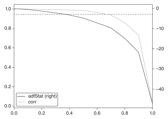
Source: Marcos López De Prado, “Advances in Financial Machine Learning”

References

[1] Cohen, I., Tian, Q., Zhou, X. S., & Huang, T. S. 2007. Feature Selection Using Principal Feature Analysis.

[2] Hamilton, J. D., & Xi, J. (Year). Principal Component Analysis for Nonstationary Series.

[3] Marcos López De Prado, “Advances in Financial Machine Learning”, 2018

[4] Massimo Guidolin, Manuela Pedio, “Essentials of Time Series for Financial Applications”, 2018