Introduction
Whenever approaching Quant Trading it is crucial to be aware that the benefit of each trade we make needs to overcome the cost of trading. Transaction cost models are a way to quantify the cost of making a trade of a given size so that the information can be used in addition to the alpha and risk model to determine the best possible portfolio to hold.
When we execute a trade, we can incur in all type of cost. Those could be financing costs to leverage our portfolio, borrowing costs to cover short positions and commission cost to exchanges and other counterparties. In addition to all of that we also pay an indirect which is the impact that our own actions have on market prices.
Commission Fees and Slippage
The first two major components of transaction costs are commission fees and slippage. Commission fees are paid to brokerages, exchanges and regulators. Usually for quantitative trading, brokerage commission fees are rather small. Indeed, given the volume of trading that quants do, they can still be extremely profitable clients for brokerages. Moreover, brokers will charge also additional fees for clearing and settlement. Given the number of trades quants usually do, this can involve a significant amount of work for brokers that will be later reflected in the commission fees they will charge. Certainly, commission and fees are not a negligible, but they are not the dominant part of transaction costs, and they are usually easy to model as they are basically fixed.
Moving forward, slippage is the change in price between the time a trader decides to transact and the time the order is actually at the exchange for execution. Slippage depends on the bid-ask spread, the security’s liquidity and volatility and the execution algorithm used. Slippage depends also on the market ecology, the participants and it needs indeed periodic recalibration in transaction cost analysis. For backtesting and portfolio optimization the following approximation is usually used:

The coefficients are usually fitted from production data. Strategies that tend to suffer the most from slippage are the trend-following ones, because they are seeking to buy and sell securities that are already moving in the desired direction. On the other hand, strategies that suffer the least from slippage, and for which it can sometimes turn even positive, are those that seek mean reversion because these strategies are usually seeking to buy and sell instruments that are moving against them when the order is placed. Higher the latency of the execution algorithm used, the more time passes before her order gets to the market and the further the price of an instrument is likely to have moved away from the price when the decision was made.
Basic Transaction Cost Models
There are four basic and most common used types of transaction cost models. Still, it is worth mentioning that the unicity of each instruments makes difficult to generalize transaction cost models. Indeed, many quants build separate transaction cost models for each instrument in the effort to improve their estimates. Usually, these models are built to evolve over time based on the trading data the quant collects from his own execution system. This means that many transactions cost model are in fact highly empirical allowing the actual, observable, recorded transaction data from a quant’s own strategy to drive and evolve the model over time.
The total cost of transactions for an instrument can be visualized as a graph with the size of the order on the x-axis and the cost of trading on the y-axis. It is generally accepted that the shape of the actual transaction cost is quadratic. Many quants decide to model their transactions cost as a quadratic function of their size of trade. While this approach can capture costs more accurately, it may become computationally expensive, leading practitioners to adopt simpler and less demanding functional forms.
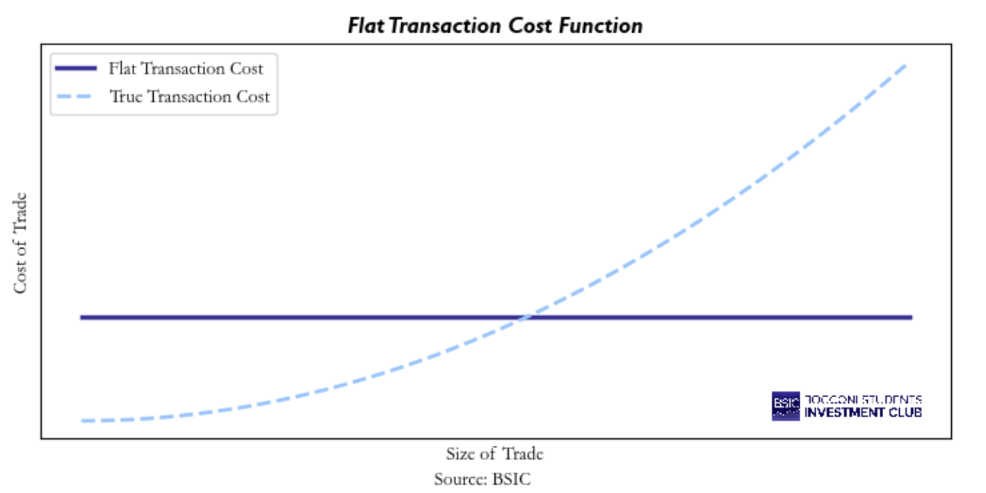
The first kind of transaction cost model is the flat model, which implies the cost is always the same, regardless of the size of the trade. This is very straightforward to implement and not at all computationally expensive. Although it is rarely correct and not widely used. The only circumstances in which such model make sense to be used is when the size of the trades are always the same and security’s liquidity and volatility remains sufficiently constant. In this case it is possible to assume the that the cost of trade will always stay the same. A chart of the flat model is shown below. Were the solid line crosses the dashed line the model is closer to a correct estimate of transaction cost. So, if this corresponds to the size of the trade normally done a flat model may not be that much problematic as long as our prior assumptions hold.
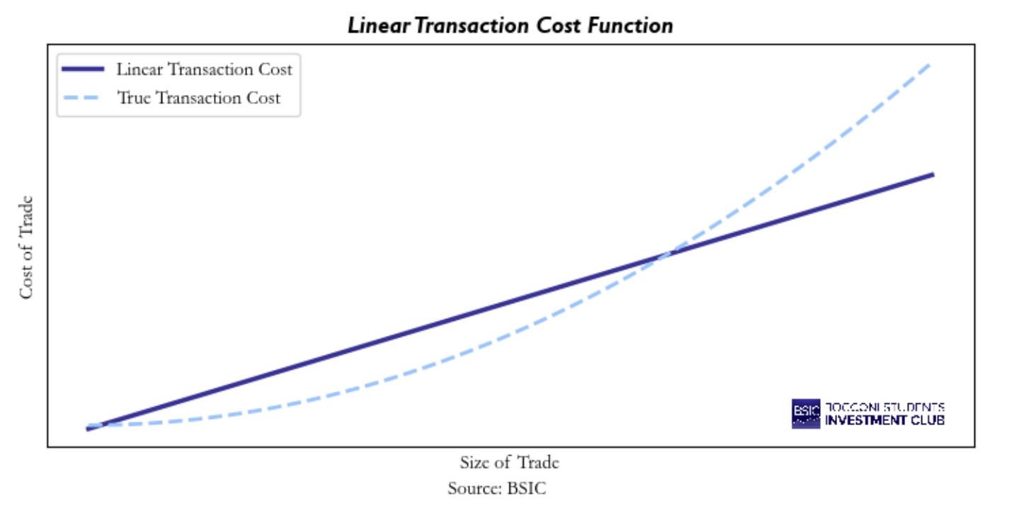
The second kind of transaction cost model is the linear model, which implies that the cost of transactions gets larger with a constant slop as the size of the trade increases. This is a better fit for true transaction costs rather than the flat model but is still mostly useful as a shortcut to building a proper model. The key trade-off in using this model is that it tends to overestimate costs for smaller trades while underestimating them for larger trades. A chart of the linear model is shown below. Again, the model I s correct when the solid line intercepts the dashed line. As with the flat model, if the size of the trade is close to those points, a linear model becomes reasonable. In any other points it remains incorrect but still appears as a better estimator than the flat model.
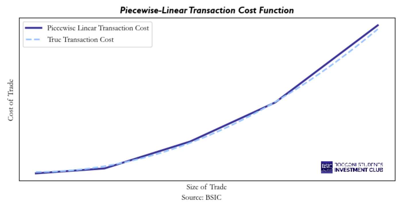
The third kind of transaction cost model is the piecewise-linear model. These types of models are used to help with precision while using reasonably simple formulas to do so. The idea behind the piecewise-linear model is that in certain ranges a linear estimation is about right, but at some point, the curvature of the quadratic estimator causes a significant enough rise in the slope of the real transaction cost line that is worth to use a new line from that point on. A chart of the piecewise-linear model is shown below. Usually, the accuracy of this type of model is significantly better than the previous ones and makes it widely used in the industry as a good medium between simplicity and accuracy.
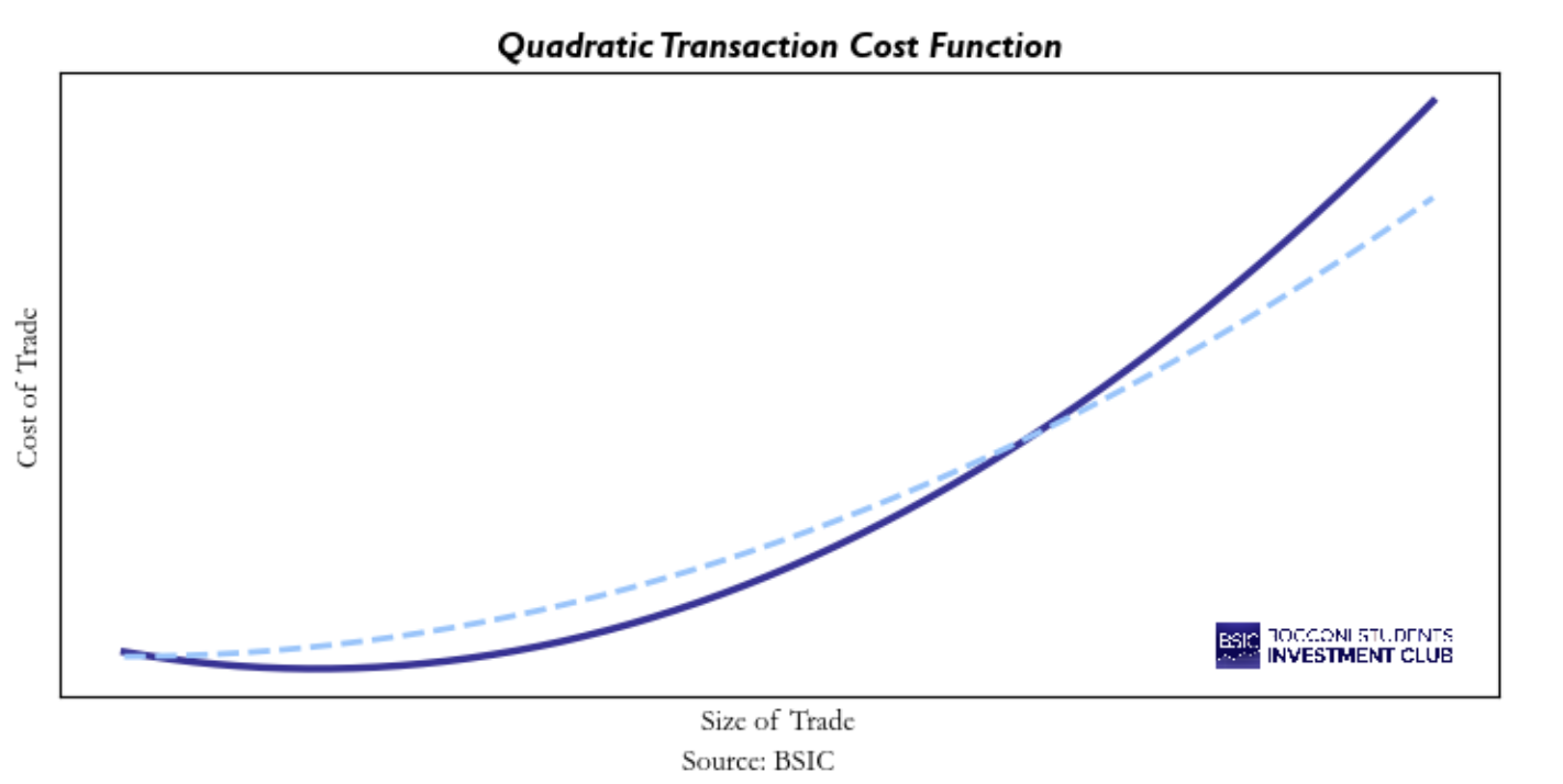
The fourth kind of transaction cost model is the quadratic model. These are computationally most intensive as the function involved is not as simple as the linear one. Although it is also the most accurate of the model, but still not perfect. Indeed, even though the shape of the function used in the model is the same transaction costs usually have also in practice, there is still discrepancy between expected and observed transaction costs. A chart of the quadratic model is shown below. The solid line is what is specified before trading, while the dashed line is what is observed empirically after trading. Causes in the divergence between estimated and realized transaction costs include: changes in liquidity or volatility of the traded security, latency, brokers and counterparties.
To conclude, the trade-off between accuracy and simplicity is something that requires a concrete judgement from who is trading. Regardless of the model used a good quant should be able to describe the cost of trading a certain instrument into its universe and should refresh periodically empirical estimates of transaction costs to ensure the model remains aligned with prevailing market conditions and to identify when further research is needed to improve it.
Market Impact
Market impact can be broadly defined as the effect that transactions made by market participants have on the price of the asset being traded. Since the core dynamic of trading is the equilibrium of supply and demand, it follows that large trades in one direction or the other have the effect of flooding the market with demand/supply and consequently move prices.
One can distinguish between “temporary” market impact and “permanent” market impact. The latter is usually interesting for actors intending to hold the asset rather than turning it around relatively quickly. The former is instead a very complex phenomenon which requires rather elaborate mathematical modelling, although the intuition is relatively straightforward intuition.
To present the topic in a clear and somewhat practical fashion the rest of the paragraph will borrow some of the concepts and notation from Paleologo [1].
We can imagine the “temporary” market impact as a shock given to the demand or supply of our asset, which shifts the price almost instantaneously (depending on factors like liquidity of the market, presence of algorithms in the specific asset etc…) and then decays through time as the market gradually goes back to equilibrium.
For this reason, we can imagine a function  as the one which regulates the instantaneous shock and a function
  as the one which models the decay of the price back to equilibrium. Therefore, if we call
  the cumulative number of shares traded up to time t and its derivative
  the shares per unit of time we can have that the expected temporary impact at time T will be given by the following:

However, despite the simple intuition behind this model, a more perilous task is to give appropriate functional form to  and
and  considering that: a) should be a (monotonically) increasing function as it represents the shock at the precise point in time (assuming would be negative for sold shares); b) should be a (monotonically) decreasing function.
The literature has tried to give several possibilities for these two functions, and we will report 2 of the more interesting alternatives from a practical point of view:
1. Obizhaeva and Wang (2013)
This model considers both a slow and a quick execution. The two functions are:


Where v is the total shares traded by all participants at a specific time  and
and  is a constant that represents the “speed” of our execution (namely, if
  our execution is “slow” and viceversa).
Plugging the two functions in the initial integral leaves us with the following solution for total trading costs  and unit costs
  :
:

![c=\kappa\tau\left[1-\frac{\tau}{T}\left(1-e^{-T}\tau\right)\right]\left(\frac{Q}{V}\right)](https://bsic.it/wp-content/ql-cache/quicklatex.com-9ba4b520214c0ec592181ea90975d45c_l3.png "Rendered by QuickLaTeX.com")
Here,  is assumed to be a constant rate of shares traded throughout the time period while
  . Normally, we can interpret the ratio
  as the participation rate of ourselves during the time interval
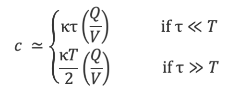
 ![\left[0,T\right]](https://bsic.it/wp-content/ql-cache/quicklatex.com-11c640b784bec6970d4bc285afb3cb84_l3.png "Rendered by QuickLaTeX.com") . It is interesting, however, that depending on our constant we have slightly different formulas for the unit costs:
. It is interesting, however, that depending on our constant we have slightly different formulas for the unit costs:
2. Almgren et al. (2005)


Where  is the volatility of the stock,
  is a constant tuned empirically at ≈ 0.6 and
  is the Dirac Delta function.
Assuming again a constant share quantity we can solve for total costs and unit costs:


Note that the unit cost is such that  , so it’s decreasing in the speed of execution.
Finite Horizon Optimization and Crossing Effect
In the previous paragraph we have outlined only some of the possible forms of our shock and decay functions. Yet, which ones to use is to be decided empirically. What we are more interested in understanding is how we can optimize our trading decisions to account for such costs. One way to do this is to solve a multi-period optimization problem using current forecasts of excess returns and plan our trades for the entire horizons. Obviously, we do not set all the trades at time 0 but rather update our forecast at each timestep and solve the optimization problem again.
Using a term proportional to trading size for transactions costs and starting from the general model outlined at the beginning of the previous paragraph, we can say the following:

where the first integral represents the transaction costs and the second is the market impact we have been talking about.
Such a model has the great advantage of being extremely flexible in the choice of the impact functions we want to use (i.e., any pair of and ) while also being able to employ all the constraints we deem necessary. The latter aren’t necessarily linear, as long as the function still appropriately maintains concavity. Yet, there’s no closed form solution (meaning a numerical solution has to be found) and convergence guarantees depend on the functional structure we decide to adopt.
An example of what an optimization problem with such a model would look like is reported by Paleologo [1]:
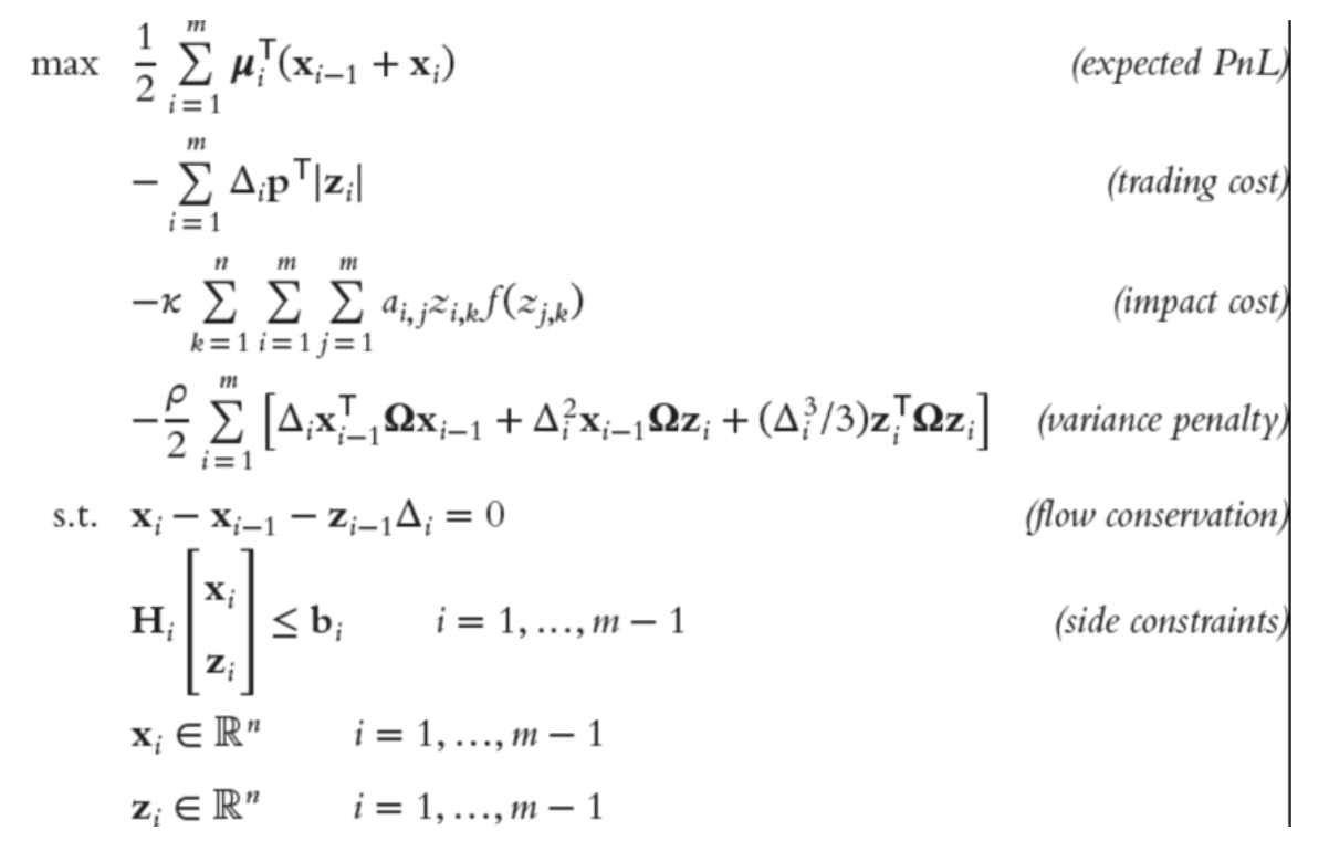
Source: Paleologo, G. “The elements of Quantitative Investing” (2025)
Obviously, there are alternatives to these models, such as single period optimization or infinite horizon problems; therefore, modelling appropriately the correct sizing and factoring in costs becomes a problem of trade-off between computational complexity and interpretability/speed of execution by the algorithm.
Conclusions
Transaction cost modelling is an essential part of quantitative trading, ensuring that strategy returns are evaluated net of realistic execution costs. Beyond static estimation, you need to keep in mind that you need to account also for market impact costs, recognizing how your own trades can influence the price of the security traded. Finite Horizon Optimization allow to determine how to schedule trades so that costs and risk are minimized. However robust transaction cost model must still evolve with the market. Regular empirical updates and thoughtful model refinement help quants maintain realistic assumptions, improve backtesting, and make more informed trading decisions under real-world constraints.
References
[1] Paloeologo, Giuseppe, “The Elements of Quantitative Investing”, 2025
[2] Paloeologo, Giuseppe, “Advanced Portfolio Management”, 2021
[3] Isichenko, Michael, “Quantitative Portfolio Management: The Art and Science of Statistical Arbitrage”, 2021
[4] Rishi K., Narang, “Inside the Black Box”, 2013


0 Comments