Introduction
In our monetary system, money markets play a crucial role in providing liquidity for financial players and are the fundamental basis of financial markets for all systemically important players. While other markets of our financial system are both well explored and documented, the money markets have stayed the least transparent while still being arguably the most important ones. In this article, we will try to explore this part of the financial world, explaining its most important aspects and outlining the consequences that funding market stress has on our financial system. We first introduce a set of rates that serve as relevant benchmarks in money markets and discuss the transactions behind them. We then discuss the hierarchy of their levels, and provide insight into the main interpretative spreads. Lastly, we discuss recurrent events driving activity in money markets.
The geography of money markets
A major aspect of money markets is repo markets: short-term collateralized cash loans, mostly overnight. In a repo trade, the borrower receives cash and posts collateral to the lender. From the perspective of the lender, this would be a reverse repo trade.
The triparty repo market is the fundamental basis of today’s repo markets, where the Fed’s primary dealers, large broker-dealers, and other relevant participants of financial markets obtain liquidity by borrowing money from asset managers with excess cash, mostly money market funds (MMFs). The most sizeable part of this market is made up of primary dealers, MMFs, and the Fed. The majority of the cash loans that are made in these markets are backed by U.S. Treasuries and other government securities, e.g. mortgage-backed securities (MBS).
Borrowers in these markets mostly act as liquidity providers for their customers who are not able to borrow in the triparty repo market, further lending out the cash obtained through their triparty repo agreements to other customers, such as hedge funds, at a higher rate in other repo markets, and thus capitalizing on the spread.
This market is called “triparty repo” as there is a third party that facilitates the transactions, thus reducing risks for lenders by taking care of the most difficult and dangerous aspects of the transactions. The only existing third-party agent for the triparty repo market in the U.S. is the Bank of New York Mellon (BNYM), which takes custody of the cash and securities of the two counterparties, but also values and monitors collateral, reports trade status, and settles balances and assets once finished. This structure allows smaller, more inexperienced players to participate in the triparty repo market. Another important aspect of this market is the fact that general collateral (GC) is used, meaning that there is no specific security that is used as collateral, but rather a basket of U.S. Treasuries or MBS, for example. The market rate negotiated between participants and at which counterparties transact is called TPR (including all types of collateral) and is effectively the rate at which primary dealers borrow cash and the rate at which asset managers, mostly MMFs, lend cash. The other significant participant of the triparty repo market is the Fed, conducting its open market operations, participating both as a borrower and a lender, being the only party to do so.
The main reference rate published by the Fed for the triparty repo rate is the Tri-Party General Collateral Rate (TGCR), which measures specific-counterparty tri-party general collateral repo transactions that are secured by U.S. Treasuries. It is also again the primary borrowing rate at which primary dealers borrow cash and the rate at which asset managers lend cash.
The Reverse Repo Facility (RRP) of the Fed, which basically sets a floor for the repo rate market through the overnight interest rate (ON RRP) it pays its lenders, which is seen as risk-free, opens two hours before the triparty repo market closes. At the RRP, eligible participants, such as primary dealers, banks, MMFs, and GSEs, can lend cash to the Fed against securities from the Fed’s portfolio, receiving the ON RRP rate. Since this is the risk-free repo rate, theoretically no one would be willing to lend to someone other than the Fed at a lower rate. However, due to the fact that not all participants in repo markets have access to the RRP, in practice rates can be lower than the ON RRP. This can also occur when huge amounts of excess cash are in the system, as the maximum amount entities can lend to the Fed stands at $160bn.
While the RRP acts as a floor for repo rates, the Standing Repo Operations (SRP) through the Standing Repo Facility (SRF) are the opposite, as they allow entities to borrow cash from the Fed through the BNYM triparty platform, acting as a ceiling to repo rates.
Next up in the opaque puzzle of different repo markets is the interdealer market known as General Collateral Financing (GCF) repo. It is characterised by dealers anonymously trading repos and reverse repos through interdealer brokers (IDBs) with each other, confirming the loan amount, the term, and the lending rate. These repos are centrally cleared by the Fixed Income Clearing Corporation (FICC).
Dealers can submit their GCF trades from 7:00 am to 3:00 pm. At 3:30 pm, the netting process begins. In netting, the FICC calculates each member’s net obligation, so either their obligation to pledge securities as collateral or deliver cash to the FICC. This essentially means that even though a counterparty could theoretically submit $100 bn in trade volume throughout the day, they could only have $5 bn in collateral that they have to pledge after the netting is conducted, as the other transactions cancel out through novation of the various repos and reverse repos that the entity has undertaken throughout the day.
After the netting, the GCF trades are cleared again through the BNYM, which is the designated clearing bank for U.S. repos, and which either wires the cash of lenders to the FICC’s BNYM clearing account or allocates the collateral of borrowers. Afterwards, it settles the obligations of each member, and the FICC’s clearing account acts as the central counterparty (CCP). It is important to note that as the pledged securities from the dealer entering the repo are only allocated to a different BNYM account, and therefore just traded within the BNYM’s book, these securities cannot be repledged into other repo segments that do not use the BNYM, to which we will come later. Another important feature the FICC and the BNYM offer is the opportunity for dealers to substitute their collateral with other eligible securities or cash until 3:00 pm, enhancing liquidity in the repo markets. This is possible for all general collateral repo markets, meaning both the triparty and the GCF repo market.
If an overnight repo initiated at time t isn’t rolled over, the trade unwinds at 3:30 pm on t+1, and the repurchase agreement is completed.
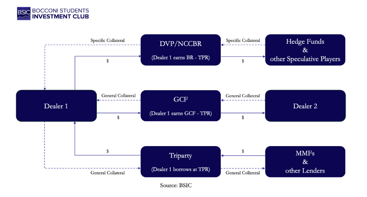
Now that we are already familiar with both the triparty repo market, the uncleared GC repo market, and the GCF, which is the cleared GC repo market, we can take a first step in looking at how the hierarchy of repo segments creates liquidity in money markets. Triparty repo lenders such as MMFs have a low risk tolerance and hence only lend to dealers with a very large capital cushion, often primary dealers. On the other hand, this means that smaller dealers cannot participate in the triparty market and hence have to borrow in the GCF market. This allows major dealers to act as market makers between different repo segments, running a so-called matched repo book. They can enter a repo in the triparty repo market and simultaneously enter a reverse repo in the GCF repo market and thus capture the spread by borrowing at TPR and lending at GCF. This can be further extended to other repo segments to which we will get to shortly.
Now that we have both introduced the triparty and the GCF repo market, there is another segment, the dealer-to-customer market, which is the largest and most important one, but also the one that remains to be the most mysterious.
Both markets we have described so far have the final intent to facilitate the trading activities of their customers. However, in dealer-to-customer markets, the “customers” range from banks and insurance companies to hedge funds and other speculative players. These markets enable speculative players to engage in activities such as leveraged trading as they are the only type of repo, in contrast to the ones mentioned earlier, where the securities are only pledged, enabling the transfer of securities between counterparties’ accounts before returning them. Here the assets, U.S. Treasuries in this case, move between participants’ accounts on Fedwire, which is the Fed’s system for electronically storing and transferring U.S. government or GSE-issued securities.
For these repo trades, a mechanism called Delivery versus Payment (DVP) is used to settle these trades. Here, both the delivery of securities and payment of cash are settled simultaneously, and the trade fails if any counterparty fails to deliver their respective obligation. In contrast to triparty repo markets, DVP repos consist of more sophisticated and risk-tolerant players like hedge funds.
The dealer-to-customer market is split in two. Part of it is cleared through the FICC’s DVP service, and the part of it that isn’t is referred to as non-centrally cleared bilateral repo (NCCBR). Both repo segments nonetheless settle via the Fedwire DVP mechanism outlined earlier.
For cleared bilateral repos, counterparties send their respective obligations to their “clearing fund”, which then goes through the FICC’s account as the FICC is the only CCP that provides centrally cleared repo trades. As a CCP, the FICC guarantees settlement of cash and securities through using its clearing funds in the case of a counterparty default. While this role of the FICC sounds like the one explained in the GCF repo market earlier, where the trades occur from dealer to dealer, over time it has also found another useful purpose in providing central clearing for dealer-to-customer markets. Together with the NCCBR market, the FICC’s DVP service facilitates upward of $5 tn in daily trade volumes.
To illustrate how the NCCBR segment works, we will demonstrate a simplified U.S. Treasuries relative value trade that is popular among hedge funds, assuming that no haircut is subtracted during the repo trades involved. We will also assume that a term repo is used as it is most common for such relative value trades. As “on-the-run” issues often have increased demand with respect to “off-the-run” securities, especially if they have very similar maturity profiles, hedge funds often try to capitalize on this by selling short the “off-the-run” in the Treasuries cash market and using the proceeds to enter a reverse repo in the NCCBR market the next morning, borrowing this exact security to deliver it to the Treasury seller. Simultaneously, the hedge fund also buys the “on-the-run” issue in the U.S. Treasuries cash market and enters a repo agreement the next morning, lending out the security and using the borrowed cash to fund its purchase. This works since most U.S. Treasury trades are settled t+1, thus giving speculators enough time to facilitate such a trade through the use of NCCBR repo markets.
Notice how the hedge fund has not used any of its own capital but has still created a gross exposure of $100 mn (assuming both the long and short position are worth $50 mn each). At t+n the term repo is completed, and we leave it to the reader to reason through the different transactions, including the interest on the term repo and term reverse repo, needed to complete the trade. This leverage through NCCBR gives hedge funds and other speculators the opportunity to profit from these minor discrepancies without using any of their own capital. If a haircut on the repo trade would have been involved, however, the hedge fund would have had to use some of its capital in order to post a margin and fund this trade. Nonetheless, the principle stays the same.
Now, a justified question would be to ask why this isn’t just facilitated by the FICC’s DVP service. While we didn’t dive deep into the specific settlement mechanics, the key reason lies beyond these details. In NCCBR, the margins, or haircuts, are negotiated “bilaterally”, which essentially means that there is no third party involved and hence results in them often being very close to zero for such relative value trades as the central constraint is dealer risk tolerance and not CCP rules. Thus, to put it simply, the FICC’s DVP service reduces the maximum leverage achievable and therefore also the potential profit for the speculator, which is why they typically prefer the NCCBR segment of the DVP market.
While this example was strongly simplified, it still illustrates how the risk-averse excess cash from an MMF can theoretically help facilitate a highly leveraged trade going through the repo hierarchy, from the triparty segment all the way to the NCCBR market. However, it is also important to note that in the middle of 2026, the uncleared dealer-to-customer market will vanish as these trades will soon have to go through the FICC’s DVP service.
Another important aspect of the GCF and DVP repo segment is that the FICC offers a “Sponsored Service” that allows smaller clients, mostly hedge funds and asset managers, who are not members of a clearing agency, to trade on the FICC’s centrally cleared platform.
Below, we created a very simplified graphic that attempts to illustrate the hierarchy of dealers, who provide liquidity by entering repos in the triparty segment and can then enter reverse repos in other repo segments. The most powerful dealers have access to every market, giving them the opportunity to borrow at the lowest rates and to lend at the highest rates, capturing the widest spreads.
 Another important aspect of getting a step closer to fully understanding repo markets is to be familiar with the daily settlement timeline for repo settlement. We will now step by step go through the most important times for the respective repo markets, going all the way back to the triparty repo market (in EST time).
At 7:00 am the BNYM’s triparty repo platform opens and trading begins to take place. Since repos are overnight loans, most participants of the triparty market already know whether they need to lend or borrow cash, which is why most of the trade agreements are done early in the morning, usually before 9:00 am. Afterwards, the counterparties communicate their trade instructions to the BNYM to finalise the details of the repo loans. The triparty market closes at 3:00 pm, and roughly two hours prior to its closing the Fed’s RRP facility opens, staying open from 12:45 pm until 1:15 pm. The Fed’s SRP, on the other hand, is open from 8:15 am to 8:30 am and from 1:30 pm to 1:45 pm every business day. At 3:30 pm after its closing, the triparty platform starts to process and settle trades. Usually, for triparty repo trades, the collateral remains in the BNYM’s settlement system overnight until the trade unwinds at 3:30 pm the next day.
Similarly to the triparty repo market, participants of the GCF repo segment also have the opportunity to submit their trades within a window ranging from 7:00 am to 3:00 pm and submit most of their trades between 7:00 am and 9:00 am. The settlement timeline is also similar as it goes through the BNYM. On the next day, the overnight loans unwind at 3:30 pm if they are not rolled over.
In our earlier explanation, we briefly talked about repo rates falling below the risk-free overnight rate at the Fed’s RRP facility. One reason is related to the time at which the participants in the reverse repo get access to their funds again, which can be only in the late afternoon when lending cash to the RRP facility. Since a lot of entities prefer liquidity over slightly higher returns, they decide to lend cash at a slightly lower repo rate rather than lock up their funds for longer.
While we have already briefly discussed the Fed’s Reverse Repo facility and the role of its corresponding ON RRP rate, it is still useful to take a closer look at the entities having access to it and to compare it to the Interest on Reserve Balances (IORB).
The ON RRP rate is the overnight rate the Fed pays in its reverse repo facility and is conducted through the triparty platform at the BNYM. Eligible counterparties include primary dealers, banks, MMFs, and GSEs. IORB, on the other hand, is simply the interest that the Fed pays on reserves held at the Fed. Here, only institutions such as U.S. commercial banks or foreign banks with U.S. branches that have master accounts can hold reserve balances at the Fed, which is a subtle but very important difference.
Notice how MMFs and GSEs like Federal Home Loan Banks (FHLBs) can use the ON RRP but cannot earn IORB. Later in this primer, we will dive deeper into the consequences this yields.
Another important factor of money markets is the Fed’s lending to other depository institutions through its discount window. The discount window often gets confused with the SRF as they both involve the Fed lending cash against collateral, but they are very different facilities in pricing, purpose, stigma, and market role. While we have already briefly touched upon the role of the SRF, we will again outline the specific differences from the discount window and explain why they are not the same.
The discount window is the Fed’s traditional emergency lending facility for banks that can be accessed by depository institutions such as commercial banks, credit unions, or basically any other institution that has a Fed master account. It primarily acts as a support tool, providing liquidity to the banking system during stress and thus preventing bank runs. Primary credit, which is the lending program to depository institutions that are judged to be in “generally sound financial condition,” has no restrictions on the use of funds borrowed. However, since the discount window is designed intentionally as a penalty rate that should be used only in an emergency, and its rate is set above the SRF rate and IORB.
While they differ from each other through the fact that certain entities such as MMFs or GSEs can use the SRF but not the discount window, another major point is the stigma surrounding the discount window. The discount window, and primary credit specifically, is a lender-of-last-resort tool that, when used, signals a sign of serious market stress and that banks are having trouble funding themselves privately.
So far, we have only specifically concerned ourselves with the U.S. money market. But since the U.S. dollar is the world’s dominant reserve currency and primary medium of exchange, we think it is justified to take a closer look at the Fed’s relationship with other participants of the financial system, especially with those that are foreign official institution (FOI) account holders. The Fed took a series of actions after both the Great Financial Crisis in 2008 and the more recent COVID-19 crisis.
After the Fed implemented the O/N RRP facility, which gave it the possibility to raise the lower limit of short-term interest rates in an ample reserves regime, it also introduced the SRF after the “repocalypse” episode of 2019, which gave it the possibility to set a hard ceiling on short-term interest rates. However, the events of 2019 threatened the stability of public institutions’ dollar portfolios, and there existed a legitimate threat of FOIs fire-selling U.S. Treasuries, which was how the FIMA repo facility was introduced. FOIs have accumulated these assets mainly through the Fed’s Foreign Repo Pool (FRP), which offers FX reserve managers of foreign governments a risk-free investment opportunity by buying U.S. Treasuries through secured repo agreements.
The FRP has enabled the Fed to be a public borrower of last resort, which is somewhat similar to the ON RRP facility setting a public instead of private dollar rate floor through the foreign repo pool rate (FRPR). Therefore, if FOIs have excess cash and no securities to invest in, they can just lend money to the Fed via the FRP, earning a small interest and thus preventing market stress that could occur from a shortage of securities on the market.
After the volatile phase in both Treasury and U.S. dollar funding markets during the COVID-19 crisis, the Fed also introduced the Foreign and International Monetary Authorities (FIMA) repo facility. The FIMA prevented FOIs from ditching Treasuries amid extreme stress and instead gave them the opportunity to temporarily swap Treasuries for dollar liquidity in the form of reserves.
Even for rivals such as China, where one would think that they would try to accelerate instability in the funding system, the FIMA has further strengthened the hold of the U.S. on our global financial system as they also need to be able to obtain U.S. dollars during serious market stress in U.S. assets, to support regional banks and other regional financial players that are in danger. Both the FIMA and FRP have further strengthened the role of the Greenback and given the Fed the ability to prevent fire sales of its assets.
In addition to the FRP and FIMA, another often less covered segment is the Fed’s role in the FX swap market. It is an additional rescue mechanism from the Fed, and through its Fed FX swap lines, the Fed is able to set a global rate limit of the overnight indexed swap rate (OIS) + 25 bp to support the global U.S. dollar FX swap market as a public dealer of last resort when private funding markets experience serious stress.
In order for our readers to understand this chapter, we will quickly cover what an FX swap is and how FX swap lines work. Through its Fed swap lines, the Fed lends U.S. dollars to a foreign central bank at the above-mentioned rate. The loan is collateralised by the currency of the foreign central bank, and when the dollar loan is repaid, the Fed returns the foreign currency. The ultimate goal of these swap lines is that foreign central banks can use the borrowed U.S. dollars to lend them to one of their local financial institutions that are in need of U.S. dollar funding, thus taking on their credit risk in the end and not the Fed’s. As foreign central banks can easily supply their own currencies, the Fed uses its swap lines to act as a lender of last resort for dollars to foreign banks as well.
Now the question arises as to why the Fed needs its swap lines if it already has the FIMA facility. While both mechanisms share the objective of preventing fire sales of U.S. Treasuries, they differ in structure and purpose. The FIMA facility allows foreign central banks to borrow U.S. dollars by pledging their existing U.S. Treasury holdings as collateral, and these operations are typically conducted on an overnight basis. Swap lines, on the other hand, often have longer maturities and allow foreign central banks to obtain U.S. dollars by pledging their own domestic currency, without drawing down their Treasury reserves. This distinction helps preserve global confidence in those central banks’ reserve positions, and to avoid spikes in offshore dollar funding rates, which could lead to second-order effects.
Not too long ago, funding stress induced through the volatility of the COVID-19 crisis left market participants unable to meet their extensive U.S. dollar needs through their usual sources such as Eurodollar markets or repos. Not only the usual FX swap dealers, but also U.S. branches of foreign banks, who are less strictly regulated, and mega banks like J.P. Morgan were unable to fill this scarcity.
Shortly after, the Fed opened its U.S. dollar swap lines, offering unlimited liquidity, which gave foreign FX dealers the opportunity to seek help from their regional central banks, who were now able to provide dollar liquidity. This brought global FX swap markets back into balance but also further underlined the Greenback’s role in the global financial system and with every further act of rescue, financial institutions that are part of the global dollar system, thus the vast majority, are growing more attached to the Fed’s role as a lender or borrower of last resort.
Hierarchy of money market rates
We first compare the levels of different rates within the same instrument category, and then introduce comparisons across types of lending and with policy rates.
Ever since the introduction of FX swap lines at the Fed, onshore and offshore rates on unsecured USD-denominated bank funding have converged. The virtual elimination of offshore dollar funding risk pushed EFFR and OBFR to trade closely to each other. The comparison of the two doesn’t reveal much.
The hierarchy of repo rates is slightly more structured. While it’s relatively difficult to make a comparison between rates in DVP/NCCBR markets and triparty and GCF repo, spreads between triparty and GCF are more interpretable. While the OFR publishes a DVP benchmark made of volume-weighted average repo rates across all collateral types, it does not collect data for NCCBR deals. Even with the DVP benchmark being available, the breadth of deals included in that rate encompasses cases in which hedge fund clients are paying the highest spreads to triparty to their dealers, but also specific-collateral repos where the security pledged as collateral is trading special. Hence a volume-weighted average rate, or perhaps even a median rate, is less informative than in other segments like triparty repo due to high dispersion.
The Office for Financial Research (OFR) collects daily volume-weighted averages of overnight TPR (excluding transactions with the Fed) across all collateral types, with its latest data release providing a time series that ends in September 2025. Data for overnight transactions in the interdealer market is provided by the DTCC’s GCF Repo Index. The DTCC’s volume-weighted average GCF rates across all collateral types are only available for the trailing 365 days, but a separate data release with rates divided by collateral type is also available. When comparing overnight TPR and GCF rates, we use the data by collateral type to maximize comparability with the TPR series.
Spreads between GCF and triparty repo have been in positive territory for most of recent history. An interpretation of GCF-Triparty spreads is related to dealer balance sheet capacity. Large dealers often borrow in triparty and lend in GCF to earn a spread. Repo intermediation weighs on dealers’ leverage ratios, so the spread must be sufficiently wide to compensate dealers for the intermediation effort. When dealer balance sheets are at capacity, less counterparties become available to perform this intermediation. Further, when dealers build up excessively large repo books, they revert to the GCF market to benefit from netting and close out excess positions. These mechanisms drive the width of the GCF-TPR spread. The Fed’s quantitative easing (from Q1 2020 to Q2 2022) and quantitative tightening (from Q3 2022 to Q4 2025) policies very likely affected the availability of reserves on dealers’ balance sheets and thus the width of the GCF-TPR spread.
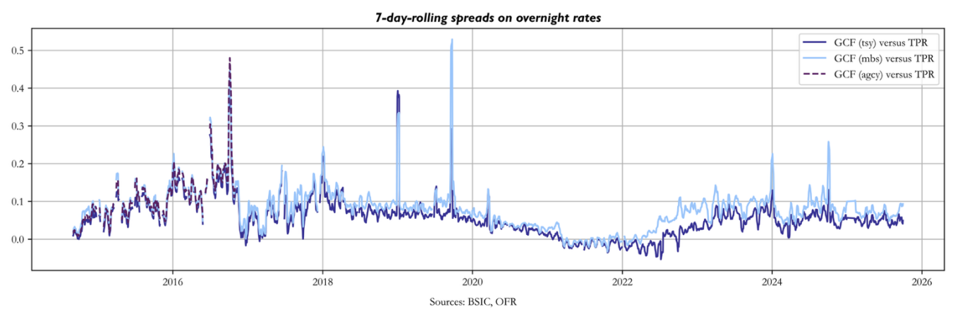
Chabot et al. (2024) attempt to provide a more accurate measure of balance sheet space compensation by measuring the spread between the average reverse repo rate charged in DVP and the average repo rate paid in tri-party, based on individual-dealer-level data. They only refer to transactions collateralized by treasury securities and adopt a specific procedure to clean out specific-collateral deals with the purpose of sourcing collateral. Their measure, named cross-market treasury repo (CMTR) spread, closely tracks the GCF-TGCR spread, but the overall trading volumes of the DVP deals going into it are much higher than those in GCF.
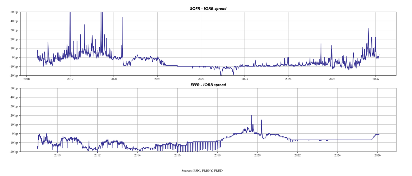
SOFR is a benchmark that the New York Fed publishes daily, and comprises deals from tri-party, GCF, and DVP repo that have treasury securities as collateral. The reports also include a distribution of the collected rates with key percentiles. SOFR can be useful when making general comparisons between repo rates across different repo markets and Fed rates, for instance. In particular, tracking the SOFR-IORB spread can be interpreted as a measure of the relative incentive for banks to engage in repo lending. Banks will likely prefer to earn IORB on their reserve balances at the Fed rather than engage in repo, but if the compensation to switch is attractive enough, they may do so.
To acquire intuition on this dynamic, we refer to a simple stylized framework presented in Clouse, Infante and Senyuz (2025) describing the optimal balance sheet size choice for a representative bank that has a reserve account at the Fed. This framework characterizes the optimal level of balance sheet size for a bank that trades reserves in the Fed funds market. The key optimality condition relates the total return of holding reserves to the total cost of funding for a bank. In particular, the representative bank will expand its reserves book until the marginal cost of acquiring an additional dollar of reserves matches the marginal return it would earn on said dollar of reserves.

The Marginal Balance Sheet Cost term should reflect, among other things, the impact of regulatory charges for an additional dollar of balance sheet size. The Marginal Liquidity Value of Reserves (MLVR), on the other hand, is unobservable and perhaps the most interesting feature of this condition. MLVR is modelled as a decreasing function of the bank’s reserves held, and it can be regarded as a precautionary buffer of reserves to guard against sudden outflows. If the bank can also choose to lend in other markets such as repo, one would expect the bank to optimize its lending in repo so that the return it earns by doing so matches the foregone return of holding reserves.

The simple framework presented above has two reality complications. Overnight unsecured funding in the Fed funds market for banks has been unincentivized by regulation after the GFC, so it’s unclear whether the MLVR term in the first identity still represents the liquidity value of additional reserves to a bank. Further, the marginal balance sheet cost may not be the same for different participants in the reserves market: to name a striking difference, US banks versus US branches of foreign-incorporated banks, since both can earn IORB, but the latter do not pay FDIC deposit insurance fees, which are influenced by balance sheet size choices. Despite these two obstacles, we can still refer to this simple framework to understand how scarce/abundant reserves are on a relative basis. When reserves are scarce, we’d expect MLVR to be relatively high, and thus we’d also expect repo rates to be above IORB.
 Switching to the perspective of money market funds (MMFs), we can perform other comparisons between rates in the repo market space and Fed rates. For example, since we know MMFs are typically net lenders in the triparty repo market, it can be meaningful to compare returns on alternative choices they have to triparty rates. Specifically, we can look at triparty rates relative to ON RRP, and falso to their level relative to yields on short-term Treasury bills. From a purely practical standpoint, repo and T-Bills are preferable to ON RRP because liquidity is readily available at any time during the day. We’d expect MMFs to locate their reserve price for repo and T-Bills around ON RRP or slightly below ON RRP to account for this relative liquidity benefit.
The ON RRP rate is the fixed floor rate set by the Federal Reserve allowing counterparties to lend liquidity to the Federal Reserve for a selected rate. The Reverse Repo Facility ties cash to the clearing house until 3:30 pm ET and, therefore, is often considered a suboptimal form of excess cash lending by the counterparties allowed to the RRP facility (i.e. primary dealers, domestic/foreign banks, GSEs, and 2a-7 money market funds).
The utility of the ON RRP rate is to act as a lower bound and maintain overnight lending within a specific range which is reviewed by the Fed every 6-8 weeks. ON RRP isn’t necessarily constant, the rate is published each morning for interested counterparties and is adjusted to account for downward pressure in the overnight lending system (for instance it can be raised by 5 bps from the target range lower bound).
Spreads between SOFR and ON RRP allow one to gauge the presence of excess reserves or collateral within the repo environment: in excess cash regimes, we often see SOFR trading around ON RRP, with exceptions. A perhaps even more indicative number to track to discern excess cash regimes from excess collateral regimes is the balance of ON RRP accounts at the Fed. As we mentioned previously, ON RRP is not a perfect substitute of tri-party repo or bills for MMFs because of liquidity differences, and hence MMFs tend to deposit heavily into ON RRP in excess cash regimes. We start by explaining the recurring effect within money markets of spikes in spreads around quarter ends to allow readers to appreciate this feature of the data.
Around quarter ends, and more generally reporting dates, dealers and other financial institutions often engage in window dressing activities. These are deliberate operational choices made by financial institutions to reduce the assets presented in their statement of financial position, in order to reduce the perceived risks of their operations, and have been significantly exacerbated by the introduction of several regulatory requirements. These activities reduce dealers’ intermediation with repo markets, effectively reducing their assets on the balance sheet and severing the ties with MMFs in the matched repo book trade operation.
To this day, there are two main constraints that dealers are facing, regulatory constraints such as the supplementary leverage ratio (SLR) and internal risk constraints such as the Value-at-Risk internal limit set by each desk. From an analysis conducted by Cochran et al. (2024) it appears that at the end of year none of the 6 G-Sibs, which also acted as primary dealers, faced threatening SLR levels. It appears that at the publishing date, primary dealers were ready to absorb the Treasury and MBS that the Fed was planning to inject in the system. The major constraint as evidenced by the paper was from internal risk models: increasing volatility, larger amounts of Treasury/MBS inventory could rapidly tighten internal risks limits and reduce dealers’ liquidity provisions.
From an accounting perspective SLR is simply the fraction of Tier 1 Capital held against the entity’s total leverage exposure. The Basel committee noticed that during the GFC a big part of regulatory failure was to be attributed to the absence of specific provisions to include off-balance sheet items when calculating bank’s minimum capital requirements. Basel III through its first pillar included off-balance sheet items such as derivatives and FX Swaps in the calculation of SLR, effectively adding some capital requirements on top of the minimum capital base required.
Interestingly, since the implementation of Basel III, US banks are required to use daily averages of repo trade operations rather than final positions when calculating (SLR). In Europe instead this change in calculation was introduced through the CRRII package, through art. 430(7) which mandated the European Banking Authority to publish the ‘Implementing technical standards’ report. Clearly stating in the Annex XI that Securities Financing Transactions (SFTs), basically repo transactions, should be accounted for as the mean of daily values for the reporting quarters when calculating the leverage ratio. This change was enforced at end of June 2021.
These changes clearly aimed to reduce the mania of big dealers to improve their SLR and decrease intermediation during quarter ends. It’s important to note that window dressing doesn’t only refer to SLR improvement: repo positions with special collateral can also increase risk-weighted assets causing considerations on internal rating-based methods MRC calculations. Furthermore, the snapshot of repo position at quarter end remains the base scenario under Basel III, and therefore, countries that haven’t adopted rules enforcing daily averaging through their banking regulation authorities could still potentially offer an incentive for regulatory window dressing to dealers.
Window dressing systems in essence affect dealers’ intermediation on quarter ends, with temporary reductions in repo activities from dealers, forcing MMFs to search for new entities to lend cash overnight. MMFs have a significant influence in the financial markets and their lending activity is constrained by an inherent risk aversion characterising their operations; the excess cash can’t totally be redirected into riskier levels of money markets. The effect is that MMFs will increase significantly their ON RRP deposited amounts and shift part of excess capacity to sponsored lending, together with Treasury bills. Since 2022, there has been a constant increase of sponsored reverse repo activity during quarter end, as these rates tend to be higher than TGCR and BGCR these could possibly be an explanation for the spikes in SOFR during quarter ends.
On the other hand, the pullback of dealers from repo activities is reflected in a higher cost of intermediation and overall higher lending and borrowing rates in the sponsored repo segment (putting upwards pressure on SOFR). Dealers in fact tend to move part of their non-centrally-cleared repo lending to central clearing to benefit from netting. Larger US custody banks that are actively pursuing sponsoring agreements increase their sponsored repo borrowing from MMFs and lend part of the funds into interdealer markets, to earn a higher spread.
Another significant set of players is that of Global Systemically Important Banks (G-SIBs). G-SIBs are banks that have a significant influence on the financial system, as classified by consultative document published by the Basel committee, and are under pervasive scrutiny. In order to maintain or improve their G-SIB surcharges, G-SIBs around year-ends tend to increase significantly their repo positions and decrease their reverse repo positions in the non-centrally cleared segment, since they are primarily lenders in this segment, and aiming to achieve more netting in GCF repo, improving the SLR ratio.
The final picture is clearly affected by a very large number of determinants. However, one thing is for certain: the reduction in intermediation of dealers clearly tightens the overall repo activity, as demonstrated by the spikes presented at quarter ends. In this sense one can also interpret the magnitude of the spikes, ignoring particular events like the failure of the Silicon Valley bank in March 2023, as the relative scarcity of reserves in the financial system, i.e. the relative liquidity shortage in the money market universe.
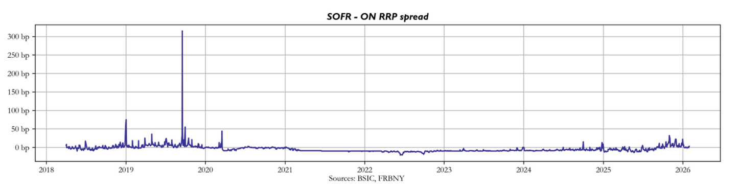
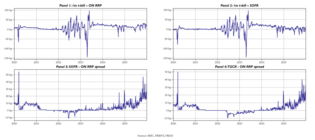 These effects can be seen in the figure in Panel 3 and 4 from 2023 onwards. We believe that the reason for negative spreads in 2022 (in Panel 1 and 2) was due to a chronic insufficient supply of T-Bills in the financial system. The series involving Treasury bill rates also show erratic behaviour around 2023, but the effect was most likely due to the debt ceiling episodes, and the fact that the data shown is for constant-maturity bill rates, which justifies a structural break in the level for observations recorded roughly 1 month before and after the X-date. For what concerns the period before 2023, the excess cash regime and relative scarcity of bills had pushed SOFR and TGCR under the ON RRP rate, to the point that MMFs started parking their excess liquidity in the ON RRP facility, reaching record highs of over $2.4 Trillion deposited in 2022 and early 2023.
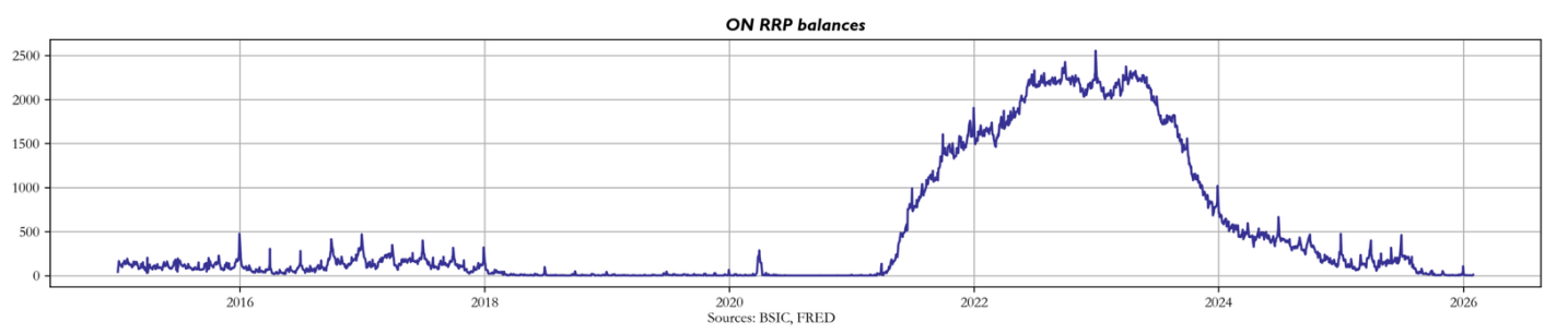
Being the ON RRP rate the floor rate set by the Fed, the balances in the facility act as an indicator of excess cash in the system. Following the ‘repocalypse’ and the global pandemic, the Federal Reserve reverted to QE injecting a massive amount of reserves in the banking system. An SLR exemption on Treasuries and reserves introduced on April 1st, 2020 (and removed on March 31st, 2021) was granted to provide dealers with more balance sheet space when intermediating transactions in Treasury markets, following the troubled episodes of March 2020 where dealers’ balance sheets had gotten to their maximum capacity, so that Treasury markets had become relatively difficult to trade in. Further, due to the massive creation of reserves with QE, and its impact on bank balance sheets, regulators had another valid motive to exempt temporarily U.S. Treasuries and bank reserves from the Supplementary Leverage Ratio (SLR) calculation. As a result, the biggest institutions flooded their balance sheet with Treasuries and reserves.
When the temporary exemption was lifted at the end of March 2021, actors had to find solutions on how to reduce their reserves: negative rates were applied on new deposits and new cash sources were refused. Dealers now flushed with funding sources were able to obtain massive discounts from counterparties which didn’t have access to the ON RRP facility, effectively pushing the TGCR and BGCR lower than the ON RRP rate, the risk-free reverse repo rate! The excess liquidity subsequently flooded into MMFs which diverted the cash surplus to the ON RRP facility as lending in the triparty segment provided lower returns.
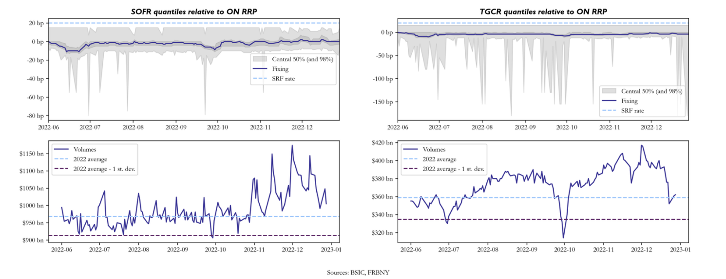 For what concerns the quarter-end episodes in 2022 where SOFR printed much lower than ON RRP (we’d expect it to print higher), it was likely because volumes in triparty repo dropped abruptly, while the volumes of deals going into SOFR exhibited a much smaller downward bump, or even increased (in July 2022). This makes SOFR more sensitive to deals in bilateral repo, where there is most dispersion.
The ON RRP facility became the Fed’s second line of defence to inadvertent rate spikes in the repo system, before Fed interventions. The Fed’s reversion to QT and the U.S. Treasury’s increase in the Fed’s Treasury General Account (TGA) coincidentally have reduced the post-pandemic excess liquidity in the money markets.
Due to their dominance in today’s funding markets, we’ve mostly talked about secured transactions for now. Unsecured money markets allow participants to make short-term loans without collateral. The borrower’s creditworthiness is essentially the main consideration when opening such positions, and therefore rating agencies are heavily consulted in the process of unsecured lending. Before the 2008 GFC commercial banks were major participants in the unsecured money markets, such that the unsecured interbank market became a term of its own. The benchmark rate for such markets was the 3-month LIBOR, which was the interest rate banks had to pay to borrow dollars on an unsecured basis for 3 months. The utility for commercial banks of such operations was the ability to expand its loan portfolio without considering deposit outflows, which affect the liability side of the B/S.
The most well-known unsecured money market is the Federal funds market, which allows banks to exchange reserves overnight on an unsecured basis. This was a useful tool for the Fed as it was able to effectively determine the supply of reserves and had a good interpretation of the overall demand for reserves. In fact, banks had to meet daily requirements on the number of reserves they hold allowing the Fed to estimate the amount that the banking system needed and adjusting the supply to maintain the fund rate within the target range.
The GFC, which primarily affected the banking sector and then propagated through the failure of insurance companies and the effects of a globally interconnected system, left many market participants wary of unsecured exposure to banks. Regulators have also made it unattractive to borrow in the unsecured money market. As a result, the interbank unsecured lending market has shrunk massively in size, and Fed Funds prints are now determined on much smaller volumes relative to prior to the GFC.
The Fed funds market still exists due to a specific system set in place since October 2008. Federal Home Loan Banks (FHLBs) have Federal reserve accounts, however when the Fed started paying interest on reserve balances FHLBs were exempted from this benefit. To gain interest on their reserves they must lend into the Federal Funds Market. Recent data from Anderson & Tase (2024) and Anderson & Na (2024) shows that FHLBs account for over 90% of the lending in the Federal funds.
The question that clearly arises is: if there is a stable (albeit smaller than in the past) supply of cash lending in the Federal funds market, who acts as a cash borrower? According to a New York Fed research report the main source of cash borrowing is U.S. branches and agencies of foreign banks (FBOs). These FBOs have access to Federal reserve accounts and are entitled to earning interest on their reserves, meaning that FBOs will earn the spread between IORB and EFFR.
It’s also important to note that FBOs, unlike domestic banks, aren’t insured by the Federal Deposit Insurance Corporation (FDIC). This limits their access to deposits, which instead are the main source of funding in the US banking system, meaning that borrowing in the Federal funds market is an important source of short-term funding. Secondly, the exclusion from the FDIC system means that FBOs don’t pay the FDIC assessment fees, meaning that FBOs face an effective EFFR that is lower than US domestic banks. The lower cost of borrowing and the different regulatory systems of leverage ratios in foreign countries make borrowing at EFFR and earning IORB an interesting proposition, since FBOs can also unwind their borrowing positions on month end or quarter end to maintain higher reported leverage ratios.
Perhaps less interestingly, we can also interpret the IORB-EFFR spread as a measure of how much compensation foreign banks with US branches demand to run IORB-EFFR arbitrage when borrowing from FHLBs. In a sense, when EFFR trades above IORB, we can also interpret it as a signal of reserve scarcity. Running EFFR-IORB arbitrage isn’t profitable any longer for US branches of foreign banks.
Event drivers of money markets
There are several factors affecting outstanding repo rates, changes in borrowing/lending over the different levels of the repo market can be explained by the relative convenience of certain actors of moving the flows they borrowed to lending in lower segments of the hierarchy to gain from the spreads present in the market. However, as supported by recent literature, one concept appears to be consistent in the last cycles of QT and QE: when the Fed enacts QT, with the reduction in its security holdings comes a reduction in bank reserves (on the liability side of the Fed’s B/S). Both effects put upwards pressure on overall repo rates, captured by the SOFR.
The relative scarcity of liquidity present in the market makes SOFR more sensitive to treasury issuance. When the U.S. Treasury injects new collateral in the market through debt issuance, demand for repo borrowing should increase, as dealers must absorb new collateral and investors require funding against higher collateral inventories. This additional demand for borrowing must face the availability of cash to lend in the repo segment. When reserve balances of depositary institutions decline, the supply of funding becomes less elastic. SOFR becomes more sensitive to new Treasury issuance.
Empirical evidence shows that during the 2017-19 QT cycle SOFR-ON RRP was more sensitive to Treasury issuance compared to the more recent post-pandemic QT episode. However, the recent re-emergence of spikes in spreads has been a common theme in money market reports.
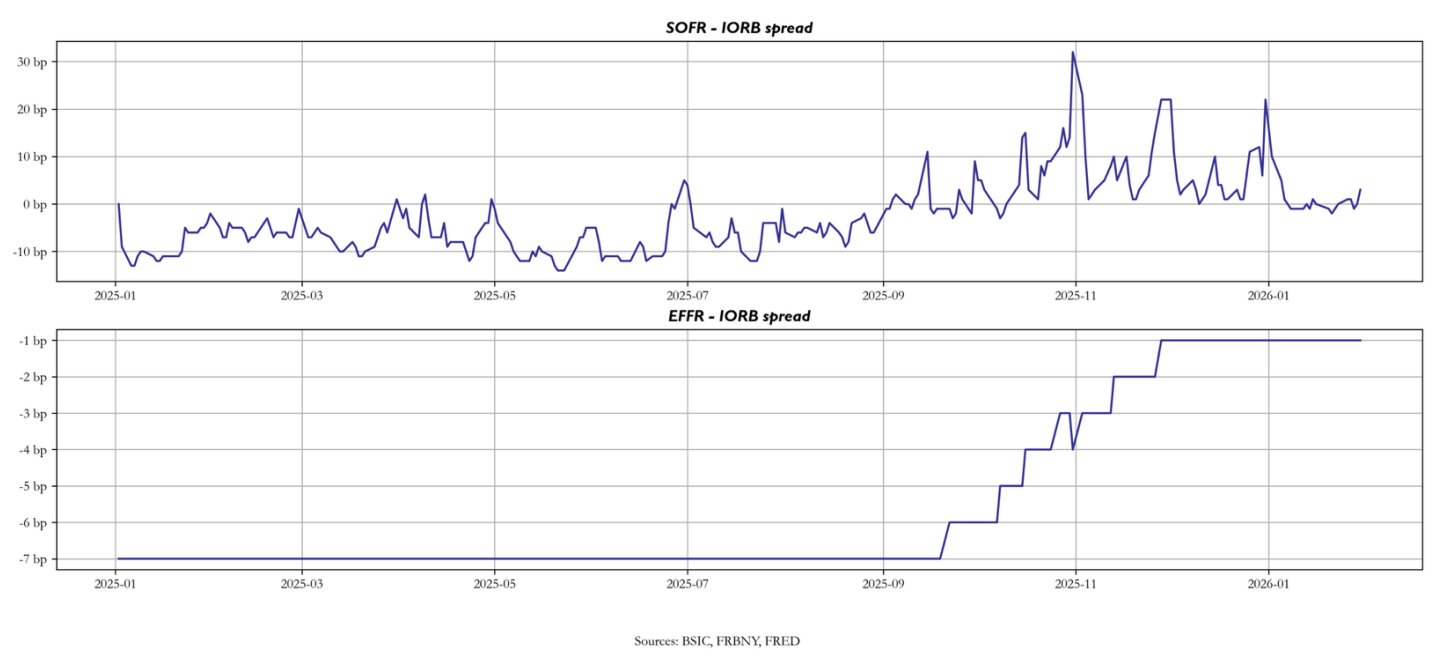
Nonetheless, we have noticed that the Fed’s most recent RMOs, T-bill purchases with newly created reserves, have greased dollar funding markets (i.e. reducing volatility and spreads), pushing SOFR just a few bps under IORB in January. The few bps of difference could be explained by the relative inconvenience of holding reserves due to major banks’ intent to front-run cuts (i.e. holding UST). However, if SOFR drifts lower, big banks may become more willing to benefit from the arbitrage offered by the fixed IORB, essentially gluing the spread. At the same time, we’ve noticed a closing of the gap between IORB and EFFR as a healthy demand of reserve liquidity.
 Money markets are highly sensitive to the reserves supply and repo funding demand. Specific fiscal events such as tax payments, Treasury issuance, government spending and TGA refills create predictable liquidity shocks that propagate through the banking system and are reflected in repo rates.
The key mechanism is the Treasury General Account (TGA), that is, the U.S. Treasury’s checking account at the Fed. Movements in the TGA effectively inject or drain reserves from the financial system. We can initially classify inflows in two types: fiscal flows related to tax payments net of transfer outlays and issuance flows related to proceeds from Treasury auctions.
Fiscal flows derive from tax payments and are thus a transfer of money from banks (and also from MMFs, as corporates liquidate their MMF holdings) to the TGA. While the Fed’s balance sheet size stays unchanged, the composition of its liability mix changes. Bank reserves are drained, and the TGA increases by the same amount. This effectively reduces funding supply, resulting in a lower reverse repo position held by MMFs which translates into lower repo borrowing (and reverse repo lending outside of triparty) by dealer banks. The effect is a higher SOFR-ON RRP spread because of a mechanical reduction in funding supply. Further, one could expect treasury yields to increase to incentivize leveraged investors bearing higher funding costs.
A very well-known episode of a funding supply shock caused by tax payments is that of 17th September 2019. A very large unwind of MMF holdings by corporates, in order to fund quarterly tax payments, created major disruptions in dollar funding markets. At the time, funding markets were in an excess collateral (scarce cash) regime. Dealers’ balance sheets were close to capacity, and lending in repo had become so profitable that it yielded more than IORB. Additionally, the Fed had been enacting QT (ended August 2019), and a TGA refill was in the making. The reserve drain from the tax payments on 17th September was the straw that broke the camel’s back. SOFR skyrocketed 325 bps above ON RRP. Market participants rushed to the fed funds market as a substitute, which couldn’t provide the necessary amount funds given how small it was relative to repo markets. The fed funds rate jumped out of the Fed’s target range for this very reason. The shock propagated to offshore markets, to the point that dollars were scarce even in FX swap markets. The Fed had to intervene with FX swap lines to settle the dust.
Issuance flows without immediate spending cause an increase in the TGA. Their effect is analogous for what concerns bank reserves, but the impact on funding markets is different. While tax flows commonly lead to funding supply shocks, issuance flows lead to funding demand shocks. Dealers and leveraged investors require funding to absorb new issuance. Hence we expect higher funding costs and spreads across markets.
TGA’s outflows necessarily have the opposite effect of refills. The US Treasury instructs the Fed to debit the TGA and the Fed consequently credits the reserve accounts of the depository institutions. The effect on the depository institutions’ balance sheet is an increase in Reserves and an increase in deposits. For instance, by the end of 2021, the U.S. government, anticipating the sharp rise in welfare, had started to fill its TGA to sustain the future cash outflows to cover the stimulus package. When the government sent funds from the TGA to the banking system there was a substantial increase in reserves. The main effects of an excessive cash regime involve a reduction in repo spreads.
It’s quite clear that the primary aim of the TGA is to support the U.S. government’s operations, such as meeting obligations and managing financing costs. Therefore, following Tax Day, the role of supporting the overall liquidity of the money market system is entrusted to the Fed, which can adjust the reserve supply in the system or expand its SRP facility usage, effectively controlling monetary plumbing.
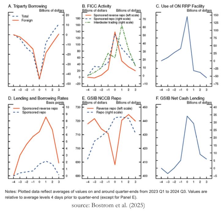
Another set of event drivers for money markets is that of quarter ends and year ends. A significant contributor to activity in these periods has historically been regulatory window dressing performed by repo dealers, for what concerns regulatory reporting of leverage ratios, and G-SIB window dressing ahead of year end to improve (or not worsen) their G-SIB surcharges.
Before the daily averaging of leverage ratios became binding for European banks, while U.S. banks had already been subject to this requirement, it’s likely that U.S. branches of European banks (and of banks in other jurisdictions) were responsible for a significant chunk of money market activity around quarter ends. For what concerns G-SIB reporting, the end-of-quarter snapshot standard is still in place even for banks in the U.S. jurisdiction. Besides letting overnight repo trades expire, the main tool these institutions have when it comes to reducing balance sheet size quickly is netting by trading more in GCF markets. Most likely, dealers also shift some of their lending appetite away from bilateral reverse repo lending (where most clients are hedge funds) and into centrally cleared repo to achieve netting. Alongside that, it’s reasonable to expect triparty borrowing to drop, as dealers cut back on intermediating from the triparty market to GCF and bilateral repo. As the key borrowers in triparty repo reduce borrowing, the key lenders (mostly MMFs) rush to sponsored repo lending, T-bills, and the Fed’s ON RRP as a last choice. We wouldn’t expect MMFs to be lenders in bilateral repo as they are arguably amongst the most risk-averse participants in money markets. Bostrom et al. (2025) inspect a sample of daily data on and around quarter ends from Q1 2023 to Q4 2024 and find evidence consistent with all of these hypotheses.
A last set of events we mention, due to its historical relevance, are U.S. debt ceiling episodes. The debt ceiling is a legal threshold setting the maximum stock of outstanding debt the U.S. Treasury can issue. For the past century, it has routinely been raised by Congress when necessary, with a few exceptions in which Congress approval was politically cumbersome. Notable recent episodes include the debt ceiling crisis of 2011 (when the U.S. government became rated below AAA for the first time) in which the ceiling was raised at the last minute, the debt ceiling crisis of 2013 (the debt ceiling was approached during a government shutdown) in which the ceiling was suspended until early 2014, and another debt ceiling crisis in 2023, in which once again the ceiling was suspended and then reset at total debt outstanding a few months after the suspension.
When the outstanding stock of debt of the U.S. Government approaches the debt ceiling threshold, the U.S. Treasury can only issue debt to roll over existing liabilities. To meet short-term obligations, the Treasury may either run down the TGA balance (if sufficiently ample) or issue “extraordinary measures” that typically involve an interruption of investments into a set of government trust funds, in order to replenish the TGA without additional issuance. In this first phase, since the TGA balance is either run down or kept flat, the impact on funding markets is usually neutral or prone to easing if a run-down occurs. A benchmark time in these episodes is the date in which the Treasury will run out of cash to meet its obligations, also known as the X-date. Approaching the X-date, it’s often common to see that treasury bills maturing after the X-date cheapen relative to those maturing before the X-date. This is usually interpreted as a risk premium for events beyond “extraordinary measures” that may happen if the debt ceiling is not raised or suspended.
The impact becomes more pronounced when the ceiling is either suspended or lifted. As the U.S. Treasury starts issuing new debt stock, without immediate outflows of cash, the TGA balance increases exerting a temporary drain of reserves from the private sector. For a more intuitive explanation, consider the following chain: following a U.S. treasury bill auction, primary dealers or any kind of investor purchasing the securities would see reserves moving from their (or their banks’) reserve account to the TGA. Further, leveraged investors will likely require repo financing to acquire the securities, and dealers running matched book trades may feed demand down to tri-party markets where MMFs will demand more compensation for their reverse repo lending.
References
- Clouse, James A., Sebastian Infante, and Zeynep Senyuz (2025). “Market-Based Indicators on the Road to Ample Reserves,” FEDS Notes. Washington: Board of Governors of the Federal Reserve System, January 31, 2025, https://doi.org/10.17016/2380-7172.3704
- Chabot, Lia, Paul Cochran, Sebastian Infante, and Benjamin Iorio (2024). “Dealer Balance Sheet Constraints: Evidence from Dealer-Level Data across Repo Market Segments,” FEDS Notes. Washington: Board of Governors of the Federal Reserve System, September 23, 2024, https://doi.org/10.17016/2380-7172.3598 .
- “Regulatory arbitrage in repo markets” (2015), Office of Financial Research, Working Paper, no 15-22, October 2015 https://www.financialresearch.gov/working-papers/files/OFRwp-2015-22_Repo-Arbitrage.pdf
- https://www.newyorkFed.org/markets/rrp_counterparties
- Erik Bostrom, David Bowman, Amy Rose, and Andy Xia (2025). “What Happens on Quarter-Ends in the Repo Market”, FEDS Notes. Washington: Board of Governors of the Federal Reserve System, June 06, 2025 https://www.Federalreserve.gov/econres/notes/Feds-notes/what-happens-on-quarter-ends-in-the-repo-market-20250606.html
- Lucy Cordes and Sebastian Infante (2025). “Repo Rate Sensitivity to Treasury Issuance and Quantitative Tightening”, FEDS Notes. Washington: Board of Governors of the Federal Reserve System, February 12, 2025 https://www.Federalreserve.gov/econres/notes/Feds-notes/repo-rate-sensitivity-to-treasury-issuance-and-quantitative-tightening-20250212.html
- Cochran, Paul, Lubomir Petrasek, Zack Saravay, Mary Tian, and Edward Wu (2024). “Assessment of Dealer Capacity to Intermediate in Treasury and Agency MBS Markets.” FEDS Notes, Board of Governors of the Federal Reserve System, October 22, 2024. https://www.Federalreserve.gov/econres/notes/Feds-notes/assessment-of-dealer-capacity-to-intermediate-in-treasury-and-agency-mbs-markets-20241022.html
- European Parliament and Council of the European Union. Regulation (EU) 2024/1623 of 31 May 2024 amending Regulation (EU) No 575/2013 as regards requirements for credit risk, credit valuation adjustment risk, operational risk, market risk and the output floor. Official Journal of the European Union L 2024/1623 (19 June 2024). http://data.europa.eu/eli/reg/2024/1623/oj
- European Commission. Annex XI: Instructions for Reporting on Leverage. Annex to the Implementing Technical Standards on Supervisory Reporting under Regulation (EU) No 575/2013 (CRR)
- Wang, Joseph (2020). Central Banking 101. Self-published, January 18, 2020


0 Comments