Technical Analysis on Steroids

Download PDF

Technical analysis is often regarded with skepticism in academic finance. It is frequently associated with delusional day traders who attempt to extract signals from price charts, relying on patterns they believe can be visually identified in candlestick formations. Over time, a vast number of technical indicators have been developed, such as moving averages, RSI, MACD, and Bollinger Bands among others; all of them are ultimately constructed using solely two features: price and volume. The core limitation of this approach is not only conceptual but also methodological. The trader must predefine the structure of the signal: for example, choosing the window length of a moving average or the threshold for an oscillator. In other words, the pattern must be specified ex-ante. If predictive structures in financial markets are nonlinear, complex, or subtle, such handcrafted indicators may fail to capture them, assuming they are present.

To address this issue, Jiang, Kelly, and Xiu (2023), in “(Re-)Imag(in)ing Price Trends” [1], propose an interesting solution: training a Convolutional Neural Network (CNN) directly on stock price chart images to forecast future returns. Specifically, the authors convert daily OHLC (open–high–low–close) data into images and feed them into a CNN, allowing the model to automatically learn predictive patterns without manual feature engineering. Their models are trained on US equities (NYSE, AMEX, and NASDAQ) over 1993–2000 and evaluated out-of-sample from 2001–2019. The results are quite remarkable. Sorting stocks into deciles based on predicted probabilities of positive returns, equal-weight long–short portfolios achieve annualized Sharpe ratios of 7.2, 6.8, and 4.9 for 5-, 20-, and 60-day image models, respectively. Notably, when restricting the universe to the 500 largest stocks, the Sharpe ratio drops to slightly above 1.

In this article, we attempt to replicate a simplified version of their approach on a much smaller scale. Due to computational constraints, we limit our universe to 20 large US stocks and focus on the period 2010–2025. Our objective is to assess whether a CNN can extract predictive information from price chart images in this reduced setting and, more importantly, whether such signals translate into portfolio returns.

87% of fund managers use technical analysis to some extent

18% of respondents indicate that technical analysis comprises a major part of their investment process

From Menkhoff, L. (2010). “The use of technical analysis by fund managers” [2]

Extracting signals from price charts

We selected 20 large U.S. equities (including AAPL, MSFT, AMZN, GOOGL, META, TSLA, JPM, NVDA, etc.) and downloaded daily OHLC and volume data from 2010 to 2025 using yfinance. To avoid data snooping, we decided ex ante that our CNN would predict returns 20 days ahead (approximately one month). Accordingly, for each stock and each date, we computed the 20-day forward return and constructed a binary target variable equal to 1 if the closing price 20 days ahead exceeded the current closing price, and 0 otherwise. This binary variable serves as the target for our classification model.

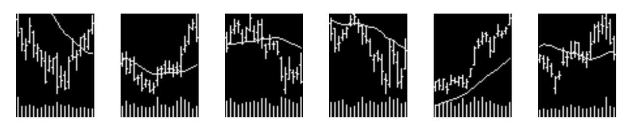
The core innovation of the paper lies in converting time-series data into images. Following a similar procedure, we generated images over 20-day rolling windows, plotting OHLC bars together with a 20-day moving average line and volume bars. Prices were rescaled within each window so that the local high and low spanned the full vertical axis, ensuring cross-stock comparability and remaining consistent with the normalization approach of Jiang et al.

The above procedure generated approximately 78,000 images, which were used both for training and testing. For reference, below are examples of randomly selected images from different stocks that were fed into the CNN.

We used images from 2010 to the end of 2018 for training, 2019 and 2020 for validation, and 2021 to the end of 2025 for out-of-sample testing. The key metrics for evaluating a classification model are the Area Under the Curve (AUC) and accuracy, defined as the ratio of correct predictions to total predictions. Over the testing set, our model achieved an AUC of 51.70% and an accuracy of 55.62%. However, 55.9% of the images in the testing set corresponded to instances of “up-movement.” This implies, frankly speaking, that our CNN performs no better than a random guess, or a coin toss, when determining whether a stock will move up or down over the next 20 days.

Nevertheless, like any classification model, the CNN produces not only a binary prediction (up or down) but also the estimated probability of a positive return (an up-movement). Notably, our CNN returned an average probability of 58%, with a maximum of 79% and a minimum of 54%. This means that, in no instance, did the model assign a probability below 50% to an upward movement. Consequently, using the standard 50% threshold, the model always “suggests” going long. This also explains why the testing accuracy coincides with the proportion of upward movements in the testing set. Clearly, the model does not support a directional trading strategy. Therefore, we tested a long–short equity strategy, following Jiang et al., to assess whether the probabilities contain a cross-sectional signal. The intuition is that if there is meaningful information in the daily ranking of predicted probabilities across stocks, it may be possible to generate returns even if the model lacks directional forecasting power.

L/S equity strategy

Over the out-of-sample period (2021-2025), the CNN produced, for each stock and each date, a probability that the stock’s 20-day forward return would be positive. We translated these probabilities into a cross-sectional trading strategy as follows:

1. On each day, all 20 stocks are sorted in descending order by
2. We select the top 5 stocks for the long leg, and the bottom 5 for the short leg
3. The resulting portfolio is equal-weighted and dollar-neutral
4. Each portfolio formed at date t is held for 20 trading days, consistent with the model’s prediction horizon
5. Because this procedure is repeated daily, after the initial 20 days we have 20 overlapping portfolios
6. Accordingly, we allocate 1/20 of the total capital to each sub-portfolio
7. The portfolio daily returns are simply the sum of the equally weighted 20 sub-portfolios returns

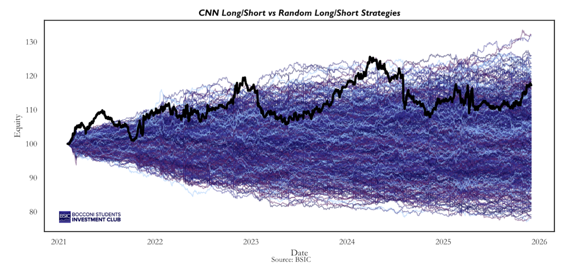
Below the equity line of the strategy over the out-of-sample period alongside the S&P 500 (volatility-matched)

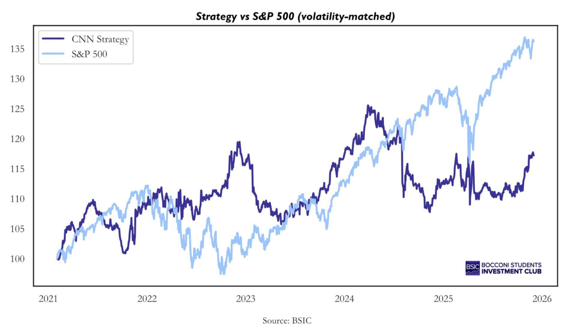The cumulative return amounts to 17.25% over the five-year period, with an annualized volatility of 8.7% and a Sharpe ratio of 0.42. This is nothing exceptional, especially considering that the S&P 500 delivered a Sharpe ratio of 0.78 over the same period. Since the plot is volatility-matched, the strategy with the higher Sharpe ratio is represented by the line lying above the other. Qualitatively, we observe that until the beginning of 2024, the CNN strategy generated higher returns and therefore exhibited a higher Sharpe ratio. Subsequently, performance plateaued, possibly indicating a regime shift that could require retraining the model. Overall, this would not be a strategy worth trading. The Sharpe ratio is already modest, even before accounting for transaction costs, which can be substantial for a L/S equity strategy with high turnover.

Nonetheless, it is interesting to analyse what the CNN is capturing, if anything at all. The correlation with the S&P 500 is -4.87%, implying a slightly negative beta of -0.02 and an annualized alpha of approximately 4%. To better understand the strategy’s exposure to systematic risk factors, we conducted a formal factor analysis. Daily factor returns were obtained from the Kenneth R. French Data Library, specifically the publicly available Fama–French Research Data 5 Factors (2×3) dataset. This dataset provides daily returns for the following risk factors:

• Mkt – rf: market excess return
• SMB: size factor (small minus big)
• HML: value factor (high minus low)
• RMW: profitability factor (robust minus weak)
• CMA: investment factor (conservative minus aggressive)

The dataset extends only through 31/12/2024, so we had to exclude the final year of the backtest from the analysis. Using OLS, we estimated the following regression:

The regression yields an R-squared of 0.7%, and all estimated betas are statistically indistinguishable from zero, suggesting that the strategy is not harvesting traditional risk factors. The residual alpha is positive and corresponds to an annualized value of 2.38%, but it is not statistically significant at any conventional confidence level.

Thus, while the strategy did not produce outstanding results, it does not appear to rely on any well-known risk factor exposures. This makes it more interesting from a research perspective than from a trading standpoint. The key question, therefore, is whether the CNN is truly capturing a meaningful signal or whether the observed positive return is simply the result of luck. To address this concern, we emphasize that we attempted to minimize data snooping as much as possible. In fact, we fixed ex-ante the stock universe, the training-testing split, the number of stocks in the long and short legs, and the 20-day forward return as the target variable for the CNN. Although this does not rule out the possibility that the results are due to chance, at least we did not iterate over multiple combinations of these parameters in search of a profitable strategy. That said, we implemented additional tests to assess whether the observed performance could be attributed to luck.

Testing robustness

First, we examined whether changing the number of long and short positions would materially affect performance. We backtested the same strategy described above using one long–short pair, two pairs, and so on, up to ten pairs. The resulting strategies are highly correlated, and all generate positive returns, although they exhibit slightly different risk-return profiles.

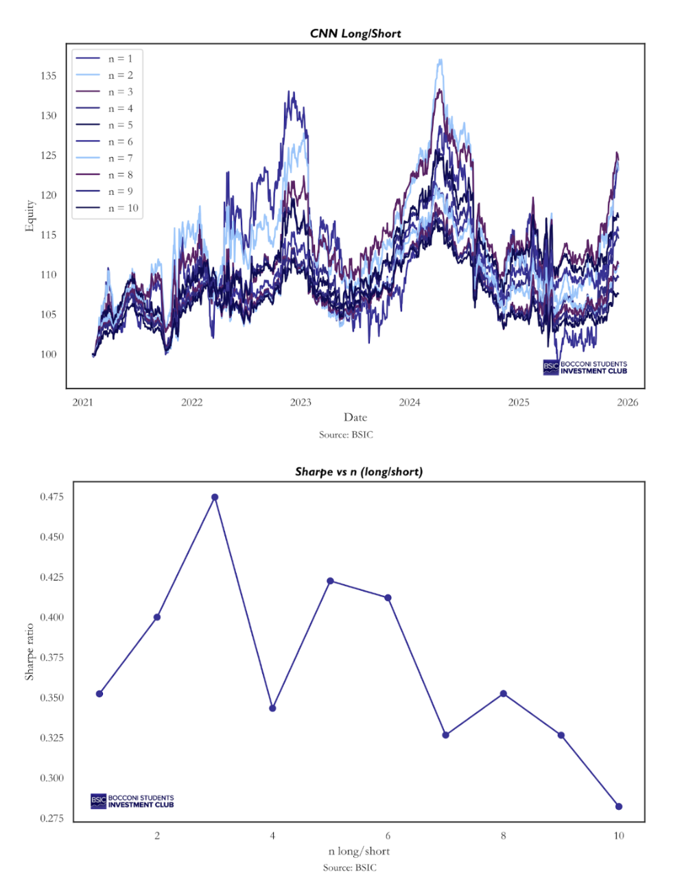
The best-performing strategy in terms of Sharpe ratio would have been going long the top 3 stocks ranked by predicted probability each day and shorting the bottom 3, while our chosen specification (5 long and 5 short positions) ranks as the second best. Our qualitative choice aimed to balance diversification with sufficient flexibility for the model to exclude stocks that may not be attractive on a given day. In this context, it makes sense that the strategy of going long 10 and short 10 performs worst, as it forces daily exposure to the entire universe, even when the signal may be weak. It is less clear why there is a sharp decline in performance when moving from 3 to 4 long–short pairs, but honestly, we do not have a definitive explanation for this.

Positions analysis

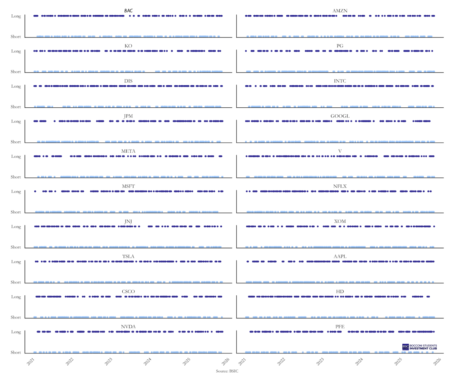
The second aspect we wanted to examine was the strategy’s exposure to individual stocks. For example, a systematic bias toward going long NVIDIA from 2023 onward could potentially explain the positive performance. To rule out this possibility, we investigated whether such anomalies were present. On this front, the strategy’s behavior appears relatively balanced. The tables below report the number of times each ticker was included in the portfolio, both on the long and on the short side.

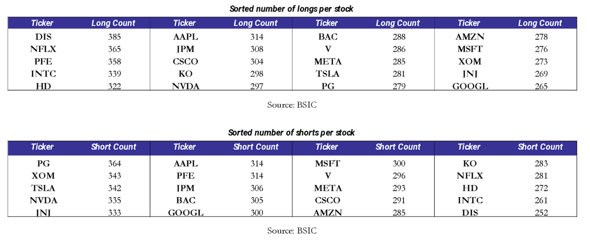While the overall allocation appears balanced, a more subtle issue is whether positions exhibit clustering over time: whether a long position in stock X tends to be followed by additional long positions in the same stock on subsequent days (and similarly for short positions). To some extent, this behavior would be both expected and desirable, as conviction in a given name may persist for several days. However, excessive clustering in a specific stock could potentially explain the strategy’s performance. The time-series analysis of positions, reported in the appendix, provides further insight. A qualitative inspection of the plot reveals some clustering in both long and short positions across individual stocks. Nevertheless, these positions appear reasonably well distributed over time, and no clear systematic bias emerges. This outcome is not surprising, since during training, the model has no information about stock identities, as it only observes images. Therefore, any persistent bias toward specific names would have been unexpected.

Monte Carlo benchmarking

A third important point is whether the strategy outperforms an appropriate benchmark. The S&P 500 is not a suitable comparator, as the CNN strategy is both market-neutral and dollar-neutral. A more relevant benchmark is a L/S equity strategy constructed on the same universe and using the same return calculation methodology. To this end, we simulated 1,000 random long–short strategies on the same 20 stocks, following exactly the same procedure described for the CNN strategy. The only difference is that, on each day, the 20 stocks are ranked completely at random rather than according to the probabilities assigned by the CNN. The intuition is straightforward: if the CNN strategy consistently outperforms the majority of these random strategies, this would suggest that the model is capturing a genuine signal. Conversely, if its performance is comparable to that of the average random strategy, the observed returns are likely attributable to luck. This simulation framework actually allows us to quantify the probability that our results are purely due to chance.

The CNN strategy consistently lies above the median of the random strategies, and by the end of the backtest only 4.3% of the random strategies achieve a higher final equity value than the CNN long–short portfolio. If trading based on the CNN probabilities were truly equivalent to trading randomly within the same stock universe, this outcome would imply that we were extraordinarily lucky. In other words, these results provide empirical evidence that the probabilities generated by the machine learning model may embed some signal. This represents the strongest piece of evidence in favor of the CNN-based strategy. However, when shifting the focus from cumulative returns to Sharpe ratios, the evidence becomes less pronounced.

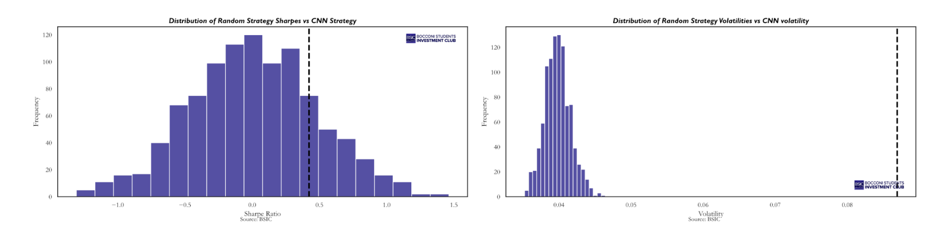In terms of Sharpe ratio, the CNN strategy outperforms 81.4% of the random strategies. Thus, when shifting the evaluation metric from terminal equity to risk-adjusted performance, the strategy moves from the top 95th percentile to roughly the top 80th percentile. This weakens the empirical evidence in its favor, as it becomes more plausible that a Sharpe ratio of this magnitude could have been obtained by chance. 

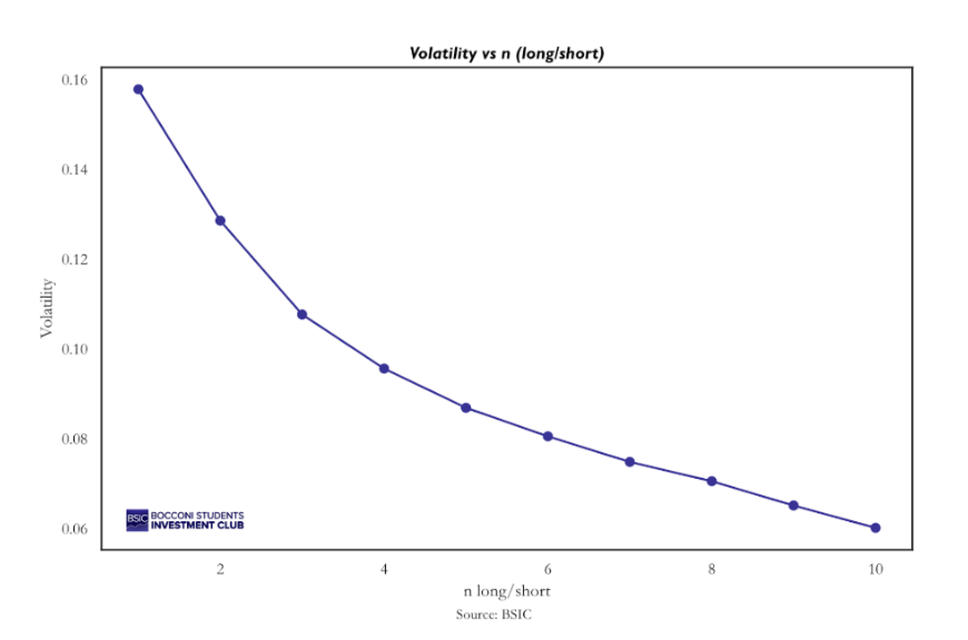
If cumulative returns are in the top 95th percentile but the Sharpe ratio only in the top 80th percentile, this implies that volatility must be higher, as confirmed by the second histogram. In fact, none of the random strategies exhibit an annualized volatility comparable to that of the CNN strategy. The mean and median volatility of the random strategies are approximately 4%, whereas the CNN-based strategy displays an annualized volatility of 8.7%, more than double. This higher volatility can be traced back to the clustering discussed in the position analysis. Persistent long or short signals lead to greater concentration in specific names compared to a fully random strategy, where such clustering is absent. As a result, diversification is reduced and the CNN strategy becomes more exposed to idiosyncratic risk associated with single names. We believe this effect is largely driven by the small universe of 20 stocks used in our analysis. With only 5 long and 5 short positions per day, the portfolio is inherently concentrated, and it is already trading 50% of the universe each day, meaning there is not much possibility to increase the number of positions. Considering a broader universe, say 500 stocks, it would be possible to increase the number of long and short positions, enhance diversification, and reduce variance. For reference, the strategy with 10 long and 10 short positions exhibits an annualized volatility of 6%, and there is a clear downward trend in volatility as the number of traded pairs increases.

Testing cross-sectional probabilities

The final test worth pursuing is whether there exists a significant positive relationship between the magnitude of the probabilities produced by the CNN and the magnitude of the 20-day forward returns it aims to predict, even if the model was trained as a classification model rather than a regression model; so, it was never exposed to the actual magnitude of the 20-day forward returns, but only to their sign (positive or negative).

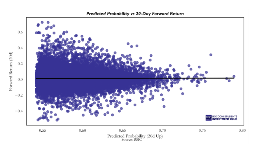
The graph speaks for itself: there is no clear relationship between the magnitude of the predicted probabilities and the magnitude of the corresponding returns, across the full dataset. This impression is confirmed by estimating the slope coefficient of a pooled regression, which yields a beta of 0.017. However, the strategy relies on cross-sectional probabilities, so what matters is whether, on each given day, the model produces a sensible ranking of stocks. In other words, we are interested in whether the cross-sectional relationship between predicted probabilities and subsequent returns is positive on average. To assess this, we estimated the following regression via OLS for each day:

This procedure yielded 1,214 daily beta estimates, with an average value of 0.033, indicating a mildly positive cross-sectional relationship. To determine whether we can reject the null hypothesis that the true average beta is equal to zero, we computed the corresponding t-statistic:

The resulting t-statistic is 1.59, corresponding to a p-value of 0.11. Therefore, we cannot reject the null hypothesis at conventional significance levels, although the result is very close to the 10% threshold. A statistically significant average beta would imply that higher predicted probabilities are associated with higher subsequent 20-day forward returns. Such a finding would constitute strong evidence in favor of the strategy, as it would confirm that the model’s probability estimates contain meaningful cross-sectional information about expected returns.

However, the formula above assumes that the beta estimates are independent from one another. In our case, this assumption does not hold. The dependent variables in the daily cross-sectional regressions are highly correlated because consecutive 20-day forward returns overlap substantially, as two consecutive observations share 19 out of the 20 underlying daily returns. To illustrate this concept, suppose we are on December 1, 2024, and we predict the 20-day forward return from December 1 to December 21. On the following day, we predict the 20-day forward return from December 2 to December 22. The returns from December 2 to December 21 are common to both windows, implying strong overlap and, therefore, non-independent beta estimates. This serial dependence is confirmed by the Auto-Correlation Function (ACF):

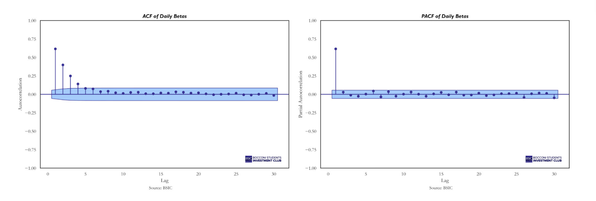Serial correlation reduces the effective number of independent observations, which in turn inflates the t-statistic and overstates the statistical significance of the test. A common correction in this setting is:

Where k denotes the sample autocorrelation of the beta series at lag , and is the truncation lag determining the maximum order of serial dependence in the time-series. In our case is 19, as consecutive betas share 19 overlapping returns. Applying the above correction we get

Recomputing the t-statistic using the reduced effective sample size yields a value of 0.73, with a corresponding p-value of 0.46, which is not even close to being significant at any confidence level.

Conclusion

In this article, we attempted to replicate in a simplified way the methodological framework introduced by Jiang et al. in “(Re-)Imag(in)ing Price Trends”, applying it to a much smaller stock universe. It is evident that a tradable strategy would require a significantly broader universe and substantial computational power. The results we obtained are far from those reported in the original paper, particularly in terms of Sharpe ratio. However, this outcome could have been expected. In the original study, the Sharpe ratio declined from approximately 6.8 when the model was trained on the full universe of NYSE, AMEX, and NASDAQ stocks to just above 1 when restricted to the 500 largest U.S. stocks. Therefore, achieving a Sharpe ratio above 1 with a universe of only 20 stocks would have been unrealistic.

Regarding our own strategy, we made a serious effort to determine whether the observed results were due to chance or whether the CNN was genuinely extracting some signal from the images. On this point, the evidence is mixed. The alpha is not statistically significant, nor is the average cross-sectional beta. On the other hand, the Monte Carlo simulation provides meaningful empirical evidence that the CNN is not trading purely at random. Nevertheless, considering the Sharpe ratios, we cannot entirely rule out the possibility that the observed performance is due to luck or chance.

Overall, our findings highlight two key insights. First, the economic value of image-based signal extraction is closely linked to the breadth of the stock universe considered. Second, while deep learning models may be capable of detecting patterns in stock price images, converting these patterns into statistically robust and economically meaningful trading strategies requires extensive data and substantial computational resources. Our simplified replication should therefore be interpreted not as a definitive validation of the CNN framework, but as an exploratory exercise that underscores both its potential and its practical limitations.

Appendix

L/S over time

References

1. Jiang, Jingwen; Kelly, Bryan; Xiu, Dacheng (2023), (Re-)Imag(in)ing Price Trends, The Journal of Finance.
2. Menkhoff, L. (2010). The use of technical analysis by fund managers: International evidence. Journal of Banking & Finance