Introduction
In this article, after a brief introduction to efficient market hypothesis and the very basics of technical analysis, we implement two different trading strategies based on moving averages and few oscillators on a wide set of equity indexes in various countries. The aim is to investigate whether efficient market hypothesis holds across markets of very different areas.
The efficient markets hypothesis
Efficient Market Hypothesis (EMH) is one of the cornerstones of financial economics. First presented by Professor Eugene Fama in 1970, EMH states that any financial asset traded in the market is always traded at its fair value, thus making impossible for investors to identify undervalued and overvalued securities and to anticipate future market trends. As soon as any new information comes in, prices immediately adjust accordingly.
The definition of EMH strictly depends on the connotation attributed to the term “fair value”. Indeed, the set of information that is meant to be used to determine the fair value of an asset can vary a lot. Therefore, three main variants of the EMH are introduced: weak, semi-strong and strong forms. In the case of weak form efficiency, the information set is composed by all data of the past market prices of the asset. In the case of semi-strong form efficiency, the information set is given by all the publicly available information, both microeconomic (dividend policy, earnings …) and macroeconomic (interest rates, inflation, exchange rates …). Finally, in the case of strong form efficiency, the market prices incorporate all the public and private information available.
Financial markets lack of strong form efficiency. As a matter of fact, the existence of insider trading is evidence that it is possible to profit from the availability of private information.
Semi-strong market efficiency is still matter of academic debate. As a general rule, the most developed and liquid financial markets enjoy semi-strong form efficiency, while often the same cannot be said about more peripheral and small markets. For instance, a large literature shows how the US markets efficiently price earnings announcements, stock splits, FED announcements as soon as the information is made public, even though some limited grey areas of inefficiency remain (e.g. IPO announcements, value anomaly, size anomaly). The presence of semi-strong form efficiency implies that fundamental analysis cannot produce consistent excess returns.
For what concerns weak form efficiency, the overwhelming majority of the academic works shows how efficiency holds in the major financial markets and in the more peripheral as well. The most basic test for weak efficiency consists in looking at the autocorrelations of market returns. In every relevant market the autocorrelation coefficients are not statistically different from zero.
Nevertheless, some contradictory results are found when more sophisticated manipulations of past prices are used to obtain signals on future market trends. For instance, in 1992 Brock, Lakonishok and LeBaron showed that, by implementing a strategy based on support-resistance levels and moving averages to produce trend inversion signals, it was possible to earn consistent excess returns on the Dow Jones from 1897 to 1986.
In addition to that, there are a number of anomalies that cast some doubts about the weak form efficiency of the major financial markets. The most significant examples are the “weekend effect” (statistically significant differences in market returns across different days of the week, with Mondays usually showing weaker performances than the second part of the week) and the “January effect” (stocks, and in particular small cap stocks, show significant better returns in January with respect to the rest of the year). These anomalies, that can be detected also in the most developed and liquid markets, find their explanation in behavioural finance in the first case and in fiscal considerations for the asset managers in the second case.
Although the theoretical credentials of trading rules are very weak, the reason why in some cases they might work is a very intriguing topic. The exploitation of these inefficiencies in the markets is the goal of technical analysis.
An introduction to technical analysis
Technical analysis is the study of market action, primarily through the use of charts, for the purpose of forecasting future price trends. Therefore, the instruments available to the analyst are basically historical data concerning prices and volumes. Technical analysis is in open contradiction to all the forms of market efficiency, as the latter implies that the current price of a security already incorporates all available data, so that it is not possible to systematically beat the market through the study of historical prices’ patterns.
On the contrary, the technician philosophy is based on three pillars. The first one is that market action discounts everything. This makes sense if you think that, given that everything possibly affecting the price (fundamentals, macro events…) is already discounted, a study of the price action is all that is needed. The second premise to the technical approach is that prices move in trends: the job of the technician is to spot new trends in their early stage. However, to discover trends and patterns there is the need for the last pillar: history repeats itself. Indeed, chart patterns and oscillators values that categorise buy or sell signals are derived from historical series. Since they worked well in the past, the technician just assumes they will work in the future as well. It is worth noting how an upward trend is not characterized by a straight positive-sloping line, but due to the nature of the markets it will be defined as a series of successively higher peaks and troughs in a given period of time.
The most widely spread ways a technician adopts to spot trends in early stages are chart patterns, moving averages and oscillators or indicators. The former are formations which appear on price charts and that have predicted value. Price patterns fall mainly in two categories: reversal (the trend in act is due to reverse) and continuation (the trend gains strength from the formation on the graph and continues its course). Examples of patterns are the “Head and Shoulders” (reversal) and the “Flags” and “Pennants” (continuation). Nonetheless, patterns are to be spotted individually by a human because of their nature, so they are not suitable for an automated trading strategy. Moving averages’ description is left to the next paragraph since they are part of the strategy we adopted. The last category of tools proves useful for the purpose of trading strategy creation: oscillators and indicators. It is crucial to note that these are to be used along with basic trend analysis, because in a sideway market situation they might provide false buy or sell signals. Most oscillators are plotted under the price chart and resemble a flat horizontal band. Generally, peak and troughs in the oscillator chart coincide with those on the price chart. Indeed, the signal the analyst tries to get from an oscillator is that when the oscillator reaches an extreme value, this signals that price may have moved too fast and it is now due for a correction. Examples of oscillators are the Relative Strength Index (RSI) and the Stochastics, which are part of the adopted strategy.
Our first strategy
The strategy we developed uses four basic indicators. These indicators are then linearly combined, and the resulting value will determine the strategy to be followed each day: if it is above a given threshold, buy the index, otherwise sell the index and keep the proceedings as cash, with returns equal to zero. The parameters that multiply each indicator have been estimated, for each index, in order to maximize the value of the portfolio on March 2015 (over an estimation window starting on 1/1/2000, or at the beginning of the series if this is later). The rest of this paragraph will provide a brief explanation of the indicators used, while on the next paragraph we will analyse the out of sample performance of the strategy from the end of the estimation window until today.
- Simple Moving Average indicator: a n-days moving average is simply the average of the closing prices of the past n days, recalculated each day. This simple tool can be used to calculate a pretty straightforward indicator that aims to detect trends in the market. Two moving averages are computed with a different estimation window. In our case, we opted for a 10-days and a 50-days moving averages. The indicator takes the value of 1 (buy) if the 10-days-MA is above the 50-days-MA, and 0 (sell) if the opposite happens. The rational is evident: if the market is bullish, then the 10-days-MA will prove to be higher than the 50-days-MA, while if the market is bearish the opposite will happen. Of course, due to its extreme simplicity this indicator cannot be used alone in order to implement a sensible trading strategy, but needs to be accompanied by other indicators that can confirm or not its signal.
- Relative strength signal: the Relative Strength Index (RSI) is an oscillator that aims at providing a signal when a given security is considered oversold or overbought. The formula to calculate it is: RSI = 100-100/1+RS, with RS = Average of n days’ gains/Average of n days’ losses. The period used for the computations is 14 days. To find the average value of positive closes, it is needed to add the total points gained on positive days and divide it for the number of days in which the security ended the session up from previous close. The RSI value ranges from 0 to 100 and an overbought signal comes in when it reaches 70 or beyond, so that the strategy will sell the index. Similarly, an oversold signal is set when the oscillator falls to 30 or below and the strategy will react by buying the index.
- Stochastic oscillator: the stochastic oscillator is used in order to determine where the last price is positioned in a range of prices over which the index traded during a given period. Indeed, as the index price is soaring, the value will be close to the upper end of the range, and vice versa. In order for the Stochastic to deliver a signal, we need to build two lines: the %K line and the %D line.
%K = 100[(Close – 14-days Low)/(14-days High – 14-days Low)]
Slow %K = 3-period simple moving average of %K
Slow %D = 3-period simple moving average of slow %K
These two lines oscillate between 0 and 100. The time frame used in the strategy is 14 days. The strategy uses the Slow Stochastic, so that slow %K and slow %D lines are to be taken into account. Alternative strategies concerning fast and full stochastics are also possible. By construction, the %K is faster than the %D line and the crossing between the two provides the bearish or bullish signal. In particular, when the %K line crosses below the slower %D, it delivers a bearish signal and the strategy sells the index. If the opposite happens, i.e. the %K breaching the %D line upwards, the strategy will buy the index.
- Accumulation distribution indicator: the aim of the Accumulator Distribution (AD) indicator is to either confirm a trend or spotting a divergence. This indicator combines the movements of the index price within the trading day and the volume of the same day. Therefore, the AD indicator does not consider the past closing prices: its aim is, indeed, not to spot a possible trend, but rather to confirm or disconfirm it. The AD indicator is built following 3 steps:
Find the Close Location Value (CLV), which is the relative “location” of the closing price with respect to the price range of the day. This is computed as follows:
CLV= [(Close – Low) – (High – Close)] ⁄ ((High – Low))
The value of this indicator is then equal to 1 if the closing price corresponds to the higher price of the day, 0 if it stays in the middle of the range, -1 if it equals the lowest price.
The CLV is then multiplied by the volume of the day, which is the number of shares traded. In our application, we used a standardized volume, equal to the volume divided by the average volume of the past 50 days of trading. In this way, we were able to produce a more stable distribution over time.
Finally, the indicator takes the value of 1 (buy), if it comes out to be higher than the 80th percentile of the distribution, 0 (sell) if it falls below the 20th percentile, and finally 0.5 (keep the position) if it lays in the middle.
The underlying idea of the indicator is as follows:
Scenario 1: the index is trending upward. If the closing price is at the top of the range with a high volume, that means that there are still more buyers than sellers and the trend should continue in the future. If, otherwise, the closing price stays at the bottom of the range, again with a high volume, this may indicate a reversing of the trend.
Scenario 2: the index is trending downward. Same (inverted) reasoning.
Empirical results
The strategy described above was implemented on 32 stock indexes taken from Western Europe, Eastern Europe, North America, South America, Asia and Africa. The out of sample window spans the period March 1st, 2015 to today. A summary of the results obtained by the strategy in the out-of-sample window is shown in the table below. In some cases, due to the absence of data on Low/High prices and/or Volume, the strategy was run without the AD indicator (indexes labelled with *), and in some cases only with the MA and RSI indicators (indexes labelled with **).
| Index Name | Index Sharpe ratio | Strategy Sharpe ratio | Standard deviations ratio | Index total return | Strategy total return | Difference in total return | Alpha | P-value |
| S&P 500 | 2,82% | 3,57% | 74% | 11,38% | 11,50% | 0,12% | 0,01% | 30,76% |
| FTSE 100 | 1,13% | 2,57% | 64% | 3,38% | 8,22% | 4,84% | 0,01% | 29,22% |
| TOPIX | 0.67% | NA | 89% | -0,36% | -11,27% | -10,91% | -0,02% | 80,89% |
| DAX 30 | 1,07% | 1,63% | 85% | 2,83% | 6,49% | 3,66% | 0,01% | 37,88% |
| STOXX EUROPE 600* | NA | 3,81% | 72% | -6,56% | 16,49% | 23,05% | 0,04% | 8,61% |
| FTSE MIB* | NA | NA | 60% | -12,60% | -13,78% | -1,18% | -0,02% | 70,34% |
| IBEX 35* | NA | NA | 72% | -7,87% | -8,76% | -0,89% | -0,01% | 61,66% |
| ARGENTINA MERVAL | 8,41% | 10,59% | 85% | 119,26% | 141,72% | 22,46% | 0,06% | 6,85% |
| ATHEX COMPOSITE | NA | 5,07% | 42% | -12,08% | 25,84% | 37,92% | 0,05% | 10,26% |
| BANGKOK S.E.T. | 0,13% | 0,05% | 93% | -1,26% | -1,40% | -0,14% | 0,00% | 51,89% |
| BIST NATIONAL 100* | 2,90% | 2,77% | 79% | 16,53% | 12,82% | -3,71% | 0,01% | 42,76% |
| BOTSWANA BGSMDC** | NA | 6,62% | 74% | -5,49% | 6,45% | 11,94% | 0,02% | 0,04% |
| CHILE IGPA | 7,90% | 9,46% | 68% | 28,55% | 23,27% | -5,28% | 0,02% | 10,29% |
| COLOMBO SE ALL SHARE** | NA | NA | 56% | -8,93% | -0,47% | 8,46% | 0,00% | 30,57% |
| EGYPT HERMES FINANC.** | 4,08% | 4,88% | 69% | 29,44% | 26,29% | -3,15% | 0,02% | 25,88% |
| FTSE LATIBEX ALL SHARE* | 1,27% | 1,70% | 51% | 2,88% | 6,58% | 3,70% | 0,01% | 39,09% |
| FTSE MALAYSIA KLCI* | NA | 1,88% | 54% | -0,83% | 2,96% | 3,79% | 0,01% | 30,71% |
| FTSE-JSE ALL SHARE | 2,49% | 4,11% | 72% | 11,23% | 15,67% | 4,44% | 0,02% | 22,32% |
| HANG SENG* | 0,97% | 2,77% | 66% | 2,34% | 10,53% | 8,19% | 0,02% | 25,82% |
| IDX COMPOSITE | 1,30% | 2,15% | 70% | 4,22% | 6,57% | 2,35% | 0,01% | 34,63% |
| ISRAEL TA 125* | 0,21% | NA | 94% | -0,97% | -10,25% | -9,28% | -0,02% | 95,43% |
| KENIA NAIROBI SE 20** | NA | NA | 43% | -38,01% | -0,93% | 37,08% | 0,01% | 9,65% |
| KOREA SE KOSPI 200 | 2,72% | 0,04% | 81% | 10,14% | -0,94% | -11,08% | -0,01% | 79,93% |
| LEBANON BLOM** | 0,62% | 5,97% | 92% | 0,85% | 26,55% | 25,70% | 0,04% | 0,09% |
| MEXICO IPC | 3,49% | 5,30% | 87% | 14,14% | 20,35% | 6,21% | 0,02% | 14,62% |
| OMX TALLIN (OMXT)** | 7,91% | 5,81% | 86% | 25,25% | 15,22% | -10,03% | 0,00% | 67,08% |
| PHILIPPINE SEI (PSEI) | 0,23% | 2,22% | 92% | -1,64% | 9,15% | 10,79% | 0,02% | 12,78% |
| PORTUGAL PSI-20* | NA | NA | 51% | -19,09% | -16,43% | 2,66% | -0,02% | 82,55% |
| RUSSELL 2000* | 2,57% | 2,16% | 81% | 12,19% | 8,16% | -4,03% | 0,00% | 48,70% |
| RUSSIAN MICEX INDEX* | 4,50% | 3,19% | 72% | 23,91% | 11,63% | -12,28% | 0,00% | 50,72% |
| SHENZHEN SE B SHARE | 1,10% | 6,85% | 65% | 2,72% | 38,29% | 35,57% | 0,06% | 3,24% |
| STRAITS TIMES INDEX L* | NA | NA | 69% | -7,80% | -7,32% | 0,48% | -0,01% | 65,24% |
| Avg | 72% | Avg | 5,67% |
Table 1: out of sample results of our first strategy (source of data: BSIC and Thomson Reuters)
The first important thing to notice is that the ratio of the standard deviation of the returns of the strategy on the standard deviation of the returns of the relative index is always less than 1. This is true by construction, since the strategy either buys the index or keeps cash, without leveraging or shorting. The last row shows that, on average, this ratio is 72%. Therefore, the strategy proposed provides less risky returns, no matter the index on which it is implemented. The Sharpe ratio is displayed only when the returns are positive, since in the opposite case it loses every significance. For this reason, the total returns of the index and of the strategy are displayed. As the table shows, on average the strategy over performed the index with a 5.67% of excess total return. At the same time, the strategy over performed the index at the end of the out-of-sample window 62.5% of times. If we look at the Sharpe ratio, however, since the strategy has a smaller volatility, this number increases to 69%. Even though these results may appear as really promising, we first need to test their significance. A binomial test of significance (not shown in the table) reveals that the p-values are 1.47% for the Sharpe Ratio, and 5.5% for the total returns. In other words, using a random strategy that has 50% of probability of outperforming the index, a higher number of successes greater than the one we obtain would have been achieved only in the 1.47% and 5.5% of the cases respectively. Another statistical test, displayed in the last two columns of the table, shows however worse results. The intercept (called alpha) of the regression of the (daily) returns of the strategy on those of the relative index is calculated. Then, a one-tailed t-test of significance is conducted. This shows than the intercept is statistically different from 0 only 19% of times at the 10% level, and 9% of times at the 5% level.
The major merit of this strategy is that it has proven to be able to recognise very well the crises. As a matter of fact, as the 2008 crash is included in the estimation window, the indicators have almost always predicted the Asian crisis of the second half of the 2015, as well as other downturns of the markets. An example taken from the Shenzhen SE B shares index is shown in the graph below.
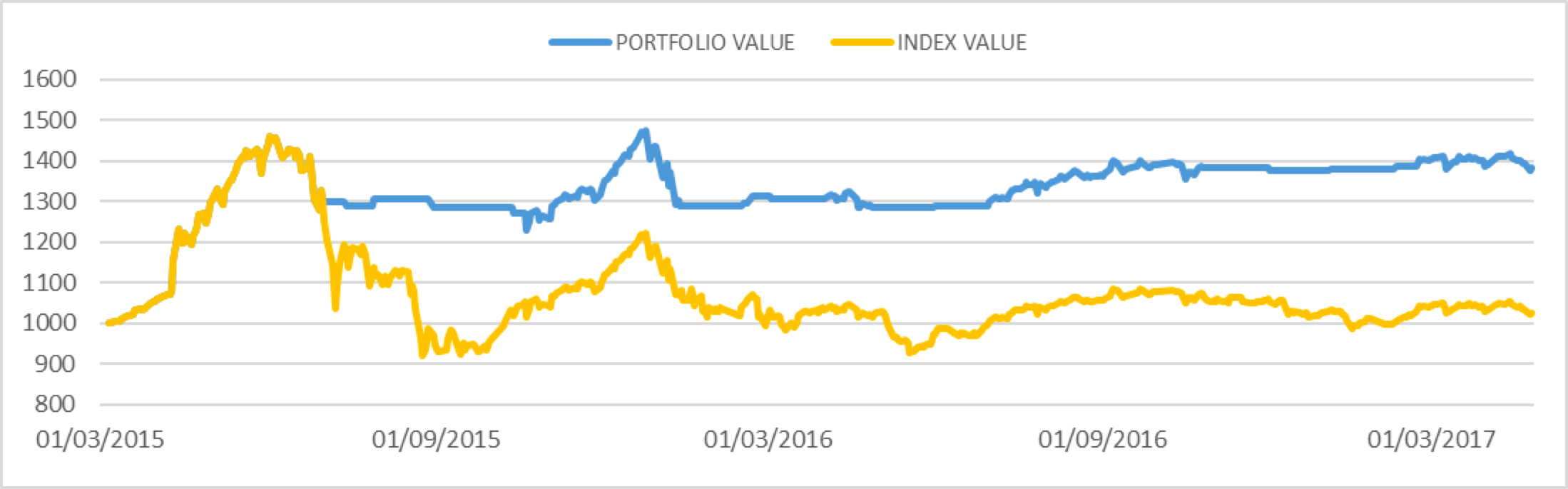 Chart 1: out of sample results of the strategy on the Shenzhen SE B, given a $1000 initial investment (source of data: BSIC and Thomson Reuters)
An alternative strategy: fuzzy logic and rolling window
We developed an alternative strategy which uses operators from fuzzy logic instead of a linear combination of the indicators.
First of all, we defined some other indicators derived from the original ones as follows.
- MA1 and MA2: MA1 is the difference between the 10-day-MA and the 50-day-MA as before. MA2 is the difference between the Closing price and the 10-day-MA. If both MA1 and MA2 are positive (so that on the price graph the 10-day-MA line is above the 50-day-MA line and the price is above both), they suggest a bullish trend.
- RSI and RSI%: one of the ways in which the RSI indicator is used is entering a long position when the RSI exits from an oversold position. To quantify the movement of the RSI indicator, we use the RSI% which is the percentage change in the RSI. We preferred the percentage change rather than the simple change in value because an increase from an oversold position will results in a higher percentage change than the same absolute increase from an overbought position. So, the interpretation of RSI% is trivial: higher the RSI%, stronger the buy signal
- SO and SD: SO is the stochastic oscillator used above, in particular the Slow-%K. Because the oscillator gives a buy signal when it increases after having decreased below 30, we define SD the difference between Slow-%K and Slow-%D, so that a positive SD when SO is below 30 can be considered a buy signal.
In the previous strategy, the technical analysis indicators were transformed into binary logic variables: 1 for “buy-index” signal and 0 for “hold-cash” signal. However, it is trivial that a higher MA1 suggests a stronger bullish trend than a lower one even if they both result in a 1 signal. A possible solution is using a variable which can assume any value between 0 and 1, so that, for example, 0.7 is a stronger buy signal than 0.2, but still lower than 1.
Here we arbitrarily choose a linear transform of the hyperbolic tangent to project an unbounded number (our indicator) into the interval [0, 1]. This function f(x) is defined as

and its plot is
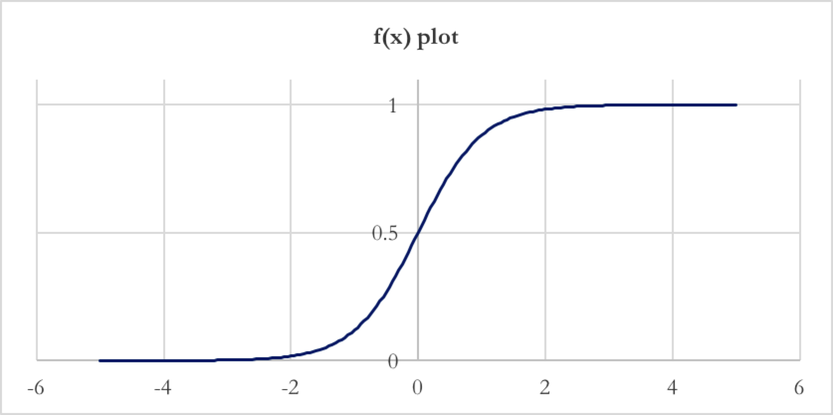
Chart 2: plot of the f(x) function (source: BSIC)
It has the useful property of being strictly increasing and having value 0.5 at f(0).
Given the different nature and possible values of each indicator, in order to get a meaningful signal, we evaluate f(x) of a proper linear transformation of the indicators as follows

where a1,a2,…,a6 are proper positive constants which will be estimated later. RSI and SO are translated by 30 so that when they are below 30 (in the oversold region) their signal is greater than 0.5.
These signals can be combined with fuzzy logic. While in Boolean logic the “truth-value” can be either 0 or 1 (false or true), fuzzy logic allows a logic variable to have all real values in the interval [0, 1]. The Boolean logic operators NOT AND OR are commonly substituted in fuzzy logic by the complement, min and max operators. However, the derivative of the min and max operators is not continuous and this fact would create issues later during optimisation. So we define the NOT and AND operators as

And the OR operator from the relation NOT [(NOT x) AND (NOT y)] = x OR y
![]()
It is trivial that these operators give the same results of Boolean logic when applied to binary logic variables.
The advantage of using these operators is that we can build a single comprehensive variable whose composition is defined ex-ante from a technical analysis technique. In particular, we define 4 strategies: one trend following, two reversal and a comprehensive one.
- Strategy 1: buy if the index is in a bullish trend. The signal Z1 is simply Z1 = SMA1 AND SMA2
- Strategy 2: buy if there is a bullish reversal, suggested by the RSI. The signal is Z2 = RSI AND RSI% (the index is exiting from the oversold region)
- Strategy 3: buy if there is a bullish reversal, suggested by the Stochastic Oscillator. The signal Z3 is Z3 = SO AND SD (very similar to the previous, but based on the Stochastic Oscillator
- Strategy 4: presence of at least one of the previous scenarios. The signal is the combination of the previous ones, so that Z4 = Z1 OR Z2 OR Z3
For each strategy, if the correspondent Z is greater than 0.5, buy the index, if not, hold a cash position.
Now, we have to estimate the parameters a1, a2, … , a6. They are estimated numerically with a simulation of the investment strategy on past values of the index. We want to consider both the return and the risk of our strategy, so the a1, a2, … ,a6 parameters must maximize the mean return of the strategy in the past with a correction for the variance of the returns.

Rs are the simulated returns of our strategy, their mean, Var(r) their variance and the positive parameter is a proxy of the investor’s risk aversion.
In order to reduce the dependence of a1, a2, … , a6 from the length of time used in the simulation, we used the weighted mean and variance of the return, with the weights exponentially decreasing for returns further in time. Because not all three indicators are available for all indexes and the optimisation is time consuming, we focused on ten of the above indexes. The parameters are estimated with 7 years of past data, then they are used to simulate an investment for the following 80 days (16 weeks of trading, about 4 months) after which they are estimated again.
For each strategy and for each index, we get a series of 0s and 1s which are the percentage of capital invested in the index for each of the n days of investment. We call this series cj and the series of index returns rj (with j= 0, …, n). The effective mean return of the strategy is

We define as a series of n random variables with mean and variance equal respectively to the sample mean and variance of cj

We call this distribution D (cj). We want to compare our effective mean return with the expected mean return obtained using instead of cj. The purpose is demonstrating that our effective return is higher than the latter by refusing the null hypothesis that the cj are randomly sampled from a distribution. So, our hypotheses are

Assuming that the are independent and the central limit theorem holds, we can calculate the p-value of our test for each strategy and index. Here are the results.
| p-value | ||||
| Index name | Strategy1 | Strategy2 | Strategy3 | Strategy4 |
| ARGENTINA MERVAL | 0% | 0% | 0% | 0% |
| BANGKOK S.E.T. | 0% | 0% | 0% | 0% |
| FTSE JSE ALL SHARE | 100% | 0% | 0% | 0% |
| HANG SENG | 0% | 0% | 0% | 0% |
| IDX COMPOSITE | 100% | 0% | 0% | 0% |
| KOREA SE KOSPI 200 | 100% | 0% | 100% | 100% |
| PHILIPPINE SEI (PSEI) | 0% | 62% | 0% | 0% |
| PORTUGAL PSI-20 | 0% | 0% | 0% | 0% |
| SHENZHEN SE B SHARE | 0% | 0% | 0% | 0% |
| FTSE 100 | 100% | 100% | 0% | 0% |
Table 2: p-values of the four strategies’ returns with respect to (source of data: BSIC)
The figures in blue are the ones for which we cannot reject the null hypothesis. As you can see, not all strategies are significant for all indexes. However, Strategy4 (the comprehensive one) is significant for all indexes, except from the Korean KOSPI. So, we focus on Strategy4 and compare it with the index.
| Index name | Index mean return (annualised) | Strategy4 mean return (annualised) | Difference in annualised return | Index Sharpe ratio | Strategy4 Sharpe ratio | Strategy4 vol / index vol |
| ARGENTINA MERVAL | 30.46% | 34.92% | 4.46% | 5.63% | 9.21% | 70.04% |
| BANGKOK S.E.T. | 9.69% | 16.99% | 7.30% | 2.96% | 7.98% | 65.09% |
| FTSE JSE ALL SHARE | 6.61% | 4.53% | -2.08% | 2.70% | 3.04% | 60.98% |
| HANG SENG | 4.30% | 10.56% | 6.26% | 1.01% | 4.02% | 61.77% |
| IDX COMPOSITE | 10.90% | 8.27% | -2.63% | 3.09% | 3.86% | 60.58% |
| KOREA SE KOSPI 200 | 5.04% | -3.90% | -8.94% | 1.46% | NA | 58.07% |
| PHILIPPINE SEI (PSEI) | 9.94% | 15.02% | 5.08% | 3.00% | 6.59% | 68.74% |
| PORTUGAL PSI-20 | -6.71% | 5.01% | 11.72% | NA | 2.46% | 56.73% |
| SHENZHEN SE B SHARE | 7.37% | 18.76% | 11.38% | 1.81% | 6.93% | 66.40% |
| FTSE 100 | 3.11% | 6.59% | 3.48% | 0.95% | 3.56% | 56.51% |
Table 3: out of sample results of Strategy4 (source of data: BSIC and Thomson Reuters)
The Korean Kospi line is highlighted since we saw that its results are not significant. The difference between the Strategy4 return and the index return is positive for almost all indexes and (excluding Kospi) the annualised mean return of our strategy is never negative. As before, because we either invest in the index or in cash, the volatility of our strategy is lower than the index one. The reduced volatility compensates the bad returns in the FTSE SJE and IDX Composite as in both cases the Sharpe ratio of our strategy is still greater than the Sharpe ratio of the index.
More relevant are the alpha delivered by each strategy and their significance.
| Index name | Alpha | p-value |
| ARGENTINA MERVAL | 0.078% | 0.0% |
| BANGKOK S.E.T. | 0.050% | 0.0% |
| FTSE JSE ALL SHARE | 0.008% | 63.9% |
| HANG SENG | 0.035% | 3.4% |
| IDX COMPOSITE | 0.017% | 22.7% |
| KOREA SE KOSPI 200 | -0.022% | 9.4% |
| PHILIPPINE SEI (PSEI) | 0.040% | 0.2% |
| PORTUGAL PSI-20 | 0.028% | 3.3% |
| SHENZHEN SE B SHARE | 0.061% | 0.0% |
| FTSE 100 | 0.022% | 6.8% |
Table 4: out of sample alphas and relative p-values of Strategy4 (source of data: BSIC)
Excluding the Korean Kospi as before, in each index the strategy delivered a positive alpha which in many cases is statistically significative at a 10% or 5% level or confidence.
Conclusions
In this article, we have first implemented a trading strategy based on four indicators, whose weights in giving signals were obtained via a point optimisation. The out-of-sample results of this strategy do not allow to detect consistent differences between the stock indexes of developed countries and those of peripheral countries. Nevertheless, we obtained surprising and unexpected good results in terms of performance on the out-of-sample window.
Given these results, we developed four new strategies obtained by implementing a more sophisticated analysis based on rolling windows optimisations and the fuzzy logic. By focusing in particular on the most comprehensive one we obtained a positive alpha in 9 indexes out of 10, 6 of which are statistically significant at the 5% level, and another one at the 10% level.
A vast scientific literature shows that technical analysis proves useless in the majority of the cases. Nevertheless, even though we acknowledge that we did not take into account any transaction cost, we have shown that relevant exceptions may arise, and produce significant alphas. To conclude, it would be interesting to conduct further analysis on different time series and indexes, as well as on the possible explanations that could be found, for instance, in the field of behavioural finance.


0 Comments