Introduction
The aim of this article is to provide a comprehensive overview of exchange-traded funds (ETFs) and to concentrate on their structure, functionality, and the factors leading to their increased use in the financial markets. Over three decades, ETFs have become a favored investment vehicle due to their cost-effectiveness, liquidity, and versatility, but still, many investors do not fully understand their operations. This paper will demystify ETFs by going through their emergence, the key participants involved, and their valuation mechanism. Alongside, it will also discuss innovations, for instance, the recent presentation of a public & private credit ETF by Apollo Global Management, Inc. and State Street, that is opening access to previously inaccessible asset classes.
ETF Popularity
ETFs, or exchange-traded funds, are funds that are publicly traded and have become very popular very fast, driven largely by their low-cost, liquidity, and flexibility, which attract both retail and institutional investors. One of the most important drivers of this boom is the low-cost advantage. The asset-weighted average fee for ETFs is about 0.30%, which is much lower than the average actively managed mutual fund fee of 0.66%. Furthermore, ETFs like the SPDR S&P 500 ETF (SPY) and the Vanguard Total Stock Market ETF (VTI), which are some of the biggest and most popular ones, have fees as low as 0.09% and 0.05%, respectively. These affordable fee charges allow investors to keep more of their returns, and consequently, ETFs are a very strong alternative to traditional investment vehicles.
The compulsion to issue the cheapest ETFs has become more and more intense year after year, and it was possible for some issuers to introduce expense ratios as low as 0.03%. For instance, the Schwab U.S. Broad Market ETF (SCHB) and the iShares Core S&P Total U.S. Stock Market ETF (ITOT) offer broad market exposure at this unusually low fee. The pricing of ETFs is referred to as a “race to the bottom,” as issuers continually cut costs in efforts to attract more assets. This drive not only serves the investors who seek to minimize fees in the long run but also triggers them to get better returns as fees are clearly a critical factor in a financial performance situation.
Liquidity is the other big reason why ETFs are so much in demand these days. ETFs are unlike mutual funds in that they are traded on stock exchanges during the day allowing for real-time data and on-the-fly trading. In the case of conventional mutual funds, the price is determined and traded only once a day at the end of the trading day. Notably, securities such as SPY are among the most traded stocks every day, with daily volumes often exceeding billions of dollars. The availability of these liquid funds gives investors, especially institutions, the option of entering and exiting positions very easily, thus keeping the huge trades of the market relatively limited.
When it comes to the competitive advantages that ETFs have, tax efficiency indeed has been a selling point with retail investors in taxable accounts. ETFs utilize an in-kind creation and redemption process, which sets them apart from mutual funds that may distribute capital gains to all investors when a large shareholder exists. For instance, when investors redeem shares of a mutual fund, the portfolio manager must raise cash by selling assets held by the fund, potentially triggering a taxable event that affects all shareholders. On the other hand, with ETFs, the tax liability is only with the seller. This can preserve the tax efficiency allowing the remaining investors to have the same advantages as before.
The diversification aspect stands out as another benefit of ETFs, and the Guggenheim Solar ETF (TAN) is a perfect illustration. This fund bundles a wide selection of solar energy companies in its portfolio, so it introduces minimal risk with single-stock exposure. When GT Advanced Technologies, an ETF holding, went bankrupt in 2014, the negative impact on the ETF was minimal, resulting in only a 0.72% drag on overall performance. This serves as an example of how ETFs can serve as a cushion when shares of companies are doing bad.
Developing an ETF
The creation of an ETF is a structured, quantitatively driven process designed to ensure the fund operates efficiently and accurately tracks its intended strategies or benchmarks with minimal tracking error. The simple process involves segmenting the ETF into either one of the two types that are primary: beta-type products or alpha-type products. By replicating a benchmark, beta-type products are meant to passively provide exposure to a specific market, index, or asset class. For instance, an ETF like the SPDR S&P 500 ETF (SPY) is a beta product that mirrors the performance of the S&P 500 index. On the other hand, alpha-type products require smart beta or active management strategies that enable them to produce excess returns by beating a benchmark.
Once the classification is established, the issuer specifies the creation unit size, which is usually 25,000 to 50,000 ETF shares, i.e., a certain notional amount like $10 million for the creation unit. This standardized block size is important for the vertices and the market-making of an ETF, and it is a prerequisite for executing large transactions without causing big swings in the underlying market.
After determining the creation unit size, the next step is the calculation of the basket constituents required for the ETF to track its benchmark. The process involves selecting assets like equities, bonds, or various other assets from different investment categories. A quantitative method is used to try to mirror the benchmark’s performance as close as possible. Additionally, after the basket selection, a thorough assessment of the liquidity and the volume is made to make sure that the fund can mint new ETF units without causing any disruptions in the market. For example, a $10 million creation unit size could be fixed by an ETF and when one of its underlying stocks trades only 10,000 shares per day, the issuer may need to downsize the weight of that stock or adjust the portfolio composition to ensure smooth trading. At this stage, the liquidity of each component is assessed to ensure the overall liquidity of the ETF with respect to the benchmark.
Rebalancing and weighting are other significant factors, especially in beta products, which aim to prevent over-concentration in some securities. Occasionally, certain stocks may outperform others, exposing a portfolio to an imbalance. For instance, one of the stocks like Apple Inc. (AAPL) may turn out to be a high performer in a technology-focused ETF ceteris paribus thus distorting the risk profile. Rebalancing gives the issuers the possibility to bring the fund back to its benchmark and maintain the desired diversification. Especially in the case of ETFs styled to mimic benchmarks, small imbalances can lead to large tracking errors.
Before the final launch, the issuer must finalize the basket composition, while having in mind the liquidity and tradability. The most illiquid stock generally determines the maximum number of shares of ETF that are either created or redeemed on a given day. If a small-cap stock lacks liquidity, the ETF’s scalability can suffer. Therefore, the ETF issuer is responsible for ensuring that the portfolio is always balanced, liquid, and tradable no matter what the market situation is.
Creation & Redemption
The creation and redemption process are crucial for maintaining an ETF’s price close to its net asset value (NAV), a mechanism that also helps to preserve market liquidity. The NAV is calculated daily by summing the total value of the ETF’s assets, subtracting its liabilities, and dividing by the outstanding shares, using the closing prices of the underlying securities.
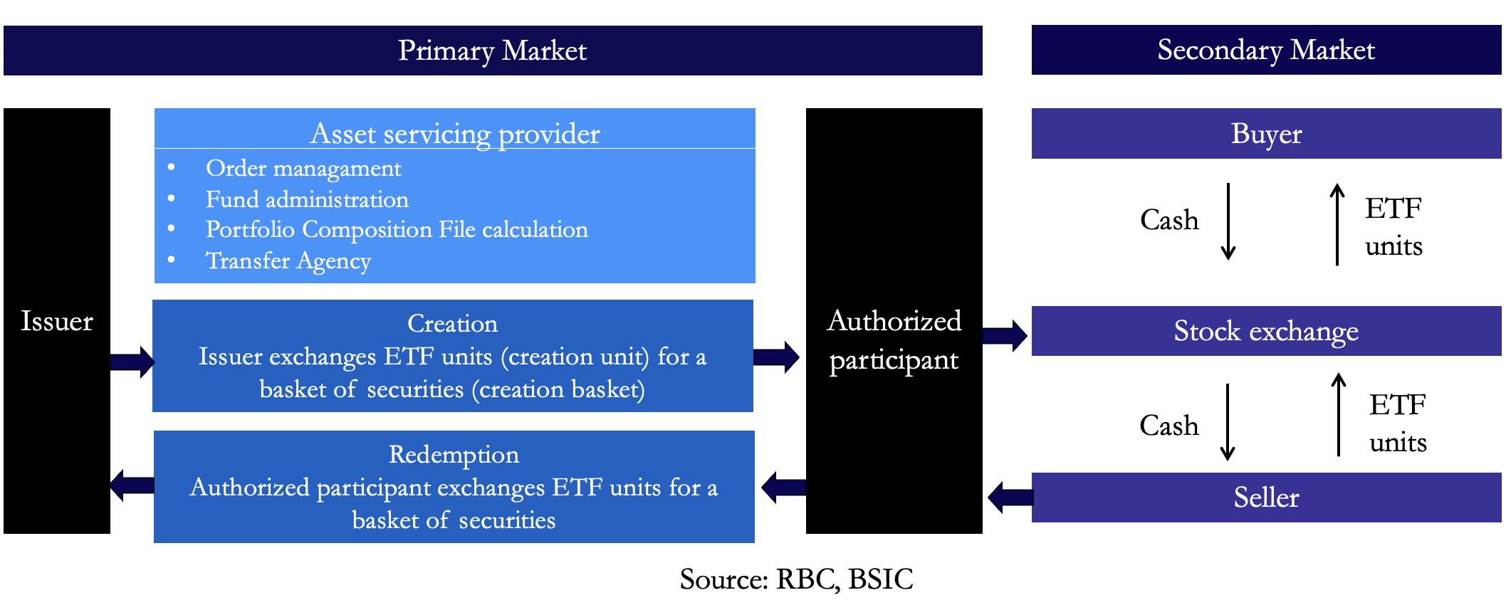
Operating within the primary market authorized participants (APs) which are typically big financial institutions like investment banks play a crucial role in maintaining this balance. APs facilitate the creation of ETF shares when demand is high and redemption when demand is low, ensuring that the ETFs market price stays aligned.
Creation occurs when the demand for ETF shares increases, and the price goes above the NAV. In this case, the APs intervene and create new ETF shares. The AP delivers a basket of underlying securities or cash (creation basket) to the ETF issuer in exchange for a block of ETF shares, known as creation unit, explained in the ‘Developing an ETF’ section. These shares are then sold on the secondary market. The AP repeats the procedure by providing additional securities to the ETF issuer in return for more ETF shares once, they have used up their inventory of ETF shares. This process leads to an increase of supply and thus brings the ETF’s price back in line with its NAV.
On the other hand, redemption occurs when the ETF price drops below its NAV due to a lower demand. In such a situation APs get ETF shares from the secondary market and redeem them by providing enough shares to form a creation unit. In return, the ETF issuer provides the AP with the equivalent portfolio of the underlying assets. This reduces the supply of ETF shares and causes the price to move back towards the NAV. To help illustrate this concept, we have included a visualization that depicts the process of creation and redemption.
This mechanism ensures, that the ETF ‘s market price remains closely aligned with its NAV. Compared to mutual funds, where the prices are determined once a day based on NAV, ETFs are still traded throughout the day, providing continuous liquidity and price transparency. This way ETFs are not only good for long-term investors, but they are also advantageous for short-term traders since they provide them with desired liquidity, transparency and cost-effective exposure to a wide range of asset classes.
The beauty of this arbitrage mechanism in the ETF is that it has created an entirely new ecosystem for trading in the markets. While in the past there were only a handful of equity indexes on which you could pursue arbitrage opportunities between baskets and futures, now there are thousands of arbitrage opportunities between baskets and ETFs.
Trading Volumes and ETF Liquidity
In this section we analyze the major differences between volume and liquidity in the ETF world, we introduce the concept of ETF implied liquidity and how money flows look like in an ETF trade.
The first key aspect is that ETF trading volume does not equal ETF liquidity. The trading volume of an ETF is a number that shows how many shares have traded of that ETF over some time in the past. The liquidity of an exchange-traded fund is based upon the underlying basket, and it is a measure of how many shares of an ETF are available to trade. Below it is shown a diagram of the liquidity function of an ETF.
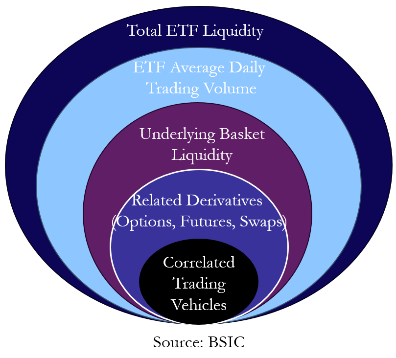
Four components of ETF liquidity work in conjunction to equal total ETF liquidity. The fist element of this function is the liquidity of the underlying basket, as determined by ETF implied liquidity. This is followed by the average daily trading volume (ADV) of the ETF which takes the number of shares that an ETF has traded over some time period in the past and calculates an average of the volume for each of those days. Other key components are the related derivatives based upon the ETF for examples, options and futures. The last components are the correlated trading vehicles: when there are products with a high correlation, participants can trade them against each other, thus driving trading volumes in each. Even though the underlying baskets are closed during the U.S. trading day, traders have developed trading relationships between EEM and VWO and DEM and trade those three products against each other.
Say, for example the ETF has an average daily trading volume of 240,800 shares, but the implied liquidity is at 11.8 million shares. If you were a portfolio manager looking to invest around $28 million in the ETF (1 million shares at $28 per share), you might initially hesitate because the fund itself only trades approximately $6.7 million worth of shares per day (240,800 shares at $28 per share). However, upon examining the underlying basket, you would see that it could potentially trade nearly $330 million per day (11.8 million shares at $28 per share), revealing much greater liquidity than you initially thought.
Quantifying the liquidity of an ETF has proven to be a challenging endeavour for market participants. There is a field available via Bloomberg called ETF implied liquidity designed to explain the most important piece of the ETF liquidity function. This field is based upon the calculation of the implied daily tradable shares (IDTS) of an ETF:

where 30-Day ADV = the Average Daily Volume over 30 days, the VP = Variable Percentage, Constituent Shares per CU = Number of shares of each stock required in the basket Creation Unit = Number of ETF shares for each basket of stocks.
The smallest IDTS becomes the constraint on how many shares can potentially be traded and is therefore the ETF implied liquidity.
Asset Under Management
Before we dive into the money flows, we need to cover another aspect that might be confusing: the relationship between volume and AUM. In fact, the actual trading volume of an ETF does not have a direct effect on the AUM. The assets under management of an ETF is the representation of how much money the fund manages. This number can change. The two factors affecting change in AUM are daily valuation changes of the fund as well as net shares created and redeemed. An ETF can trade a tremendous number of shares in a given day, but if that trading does not lead to net creations or redemptions, then the AUM can remain constant.
Take the example of an ETF arbitrage firm selling a particular ETF all day and buying baskets against it to hedge. In this example, the buyer of the ETF shares was another ETF arbitrage firm that was buying the ETF and selling the basket. At the end of the day, the firm that had been selling the ETF put in a creation order of 10 units to flatten its position. The firm that had been buying the ETF submitted a redemption order of the same size to flatten its own position. In this scenario, the ETF exhibited a very high trading volume on the day, but its net assets do not change.
Money flows of the Buyer
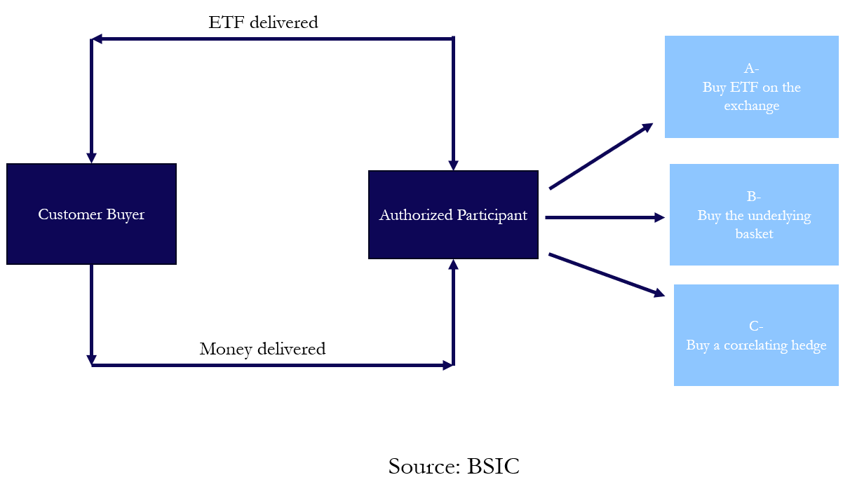
Subsequently, let’s explore how money flows in an ETF transaction, focusing on a situation where the customer is a buyer. The customer has transacted with the AP buying the ETF. Only three scenarios can then take place. In scenario A (figure below), the AP, acting as an agent, went out and bought the ETF on the exchange for the client. In scenarios B and C, the AP was providing liquidity and acted in a principal capacity. The AP sold the ETF shares to the client. APs have two choices to hedge the position. They can either buy the exact basket of the ETF, if it is trading at the same time as the ETF trade, or they can buy some other correlating asset that they use to hedge their short position in the ETF. In case A, the AP ends up buying the ETF on the exchange, on the client’s behalf. In this case, an AP is not required to do anything further because it is merely a middleman between the market and the customer. What is happening, however, is that the AP probably is buying the ETF shares from another liquidity provider somewhere along the order flow chain. At some point, that order flow gets into a scenario like that of case B.
In case B, the AP sells the ETF to the customer and can buy the underlying basket that replicates the ETF. The position on the books of the AP will be short the ETF and long the basket. Then the AP would process a creation with the issuer. This would require the AP to deliver the shares that it is long of the underlying basket to the issuer; and it would in turn receive the shares of the ETF. The AP’s position would be flat, and the issuer would have increased the shares outstanding in the fund, simultaneously increasing the AUM.
In case C, the AP buys some correlating hedge that tracks the ETF well. Since doing so implies that there will be financing charges in maintaining the long hedge and short ETF position, this is ideally a short-term solution. At some point in the future, the AP either intends to unwind the short ETF position and the hedge or will want to exchange the hedge for the basket of underlying stocks and then proceed to do a creation.
In summary, we can say that rather than buying a piece of the assets already in the fund, we are receiving liquidity from someone who will pursue a creation to increase the fund’s shares outstanding and AUM.
In the case of someone shorting an ETF, typically an AP will go out and do a short creation of the ETF to facilitate the stock loan. This means the AP will borrow the underlying basket and deliver it to the issuer who will in turn deliver out the ETF shares (increasing the shares outstanding), which can then be lent to the end client.
Market Participants
In order to gain a broad view of the major players in the ETF market, it is necessary to discuss the different types of LPs. The first player we want to discuss are investment banks, who typically have two areas that handle the facilitation of ETF order flow: the institutional ETF trading desk and the intermediary trading desk. The Institutional ETF Trading Desk is typically a feature of the equities or equity derivatives departments and works in conjunction with the equity derivatives group, portfolio trading, and institutional sales. This desk typically handles all the institutional customer businesses revolving around ETFs. The main functions are: committing firm capital to facilitate block trades in the secondary market, dealing in the primary market doing creations and redemptions as authorized participants (APs), and using firms’ trading infrastructure to access the underlying ETF liquidity for customers.
The second desk is the Intermediary Trading Desk which has evolved with the adoption of the ETF product line. This desk handles order flow from the wealth management and private banking businesses. Typically, this desk operates on an agency-only basis and facilitates client orders by either using in-house algorithms or sourcing liquidity from various market makers. It is not a profit center but rather a service that provides access to available liquidity in the market.
Large participants in terms of number of traders are also made by proprietary ETF market-making firms. These proprietary shops are responding to order flow and therefore are focusing where the order flow is. These shops do better in names where there are fewer participants, wider spreads, and more opportunities for arbitrage.
A subset of proprietary trading firms are LMMs who pursue similar businesses: arbitrage between the ETF and its respective basket. However, LMMs are registered with the stock exchange in a partnership through which they agree to meet minimum liquidity requirements for which they enjoy a modified fee structure received from the exchange.
High-frequency players have become another liquidity source by creating even more volume in many ETFs. They are using models looking at volatility and expectations for future moves to make small amounts in incredibly small time periods, even down to microseconds. Their existence and growth highlight the diversity of product uses resulting in the greater development of the ETF business.
The last type of liquidity provider has developed in recent years. This newer type of liquidity provider is called a “liquidity aggregator.” They evolved from interdealer brokers (IDBs), who used to stand between brokers who want to swap positions for certain reasons. Now, they stand between a host of market makers, proprietary and customer-facing desks, and the end ETF user. They use their long-standing relationships with the market makers to put an order into competition and get the best price. If a client does not have the market-making relationships or trading landscape acumen, liquidity aggregators can offer much value in execution.
ETF Valuation
Exchange-Traded Fund (ETF) valuation is an essential task for the accuracy and effectiveness of the financial markets where ETFs are bought and sold. The valuation policy guarantees that the ETF’s value is in the right spot and that underlying securities’ worth is correctly reflected in the ETF’s price. Two key indicators of this value are the NAV and IIV. The NAV provides the most accurate account of the true worth of an ETF at the end of the trading day. However, throughout the day, investors depend on the IIV (intraday indicative value), also called the indicative optimized portfolio value (IOPV) which is a real-time valuation of the ETF’s value that takes the latest prices of the underlying assets into consideration.
The NAV calculation formula of an ETF can be written as follows:

This equation mainly aggregates the value of each security among the ETF elements and adds the cash holding factor, and after that, converts all into a per-share basis, which is calculated by dividing the shares of ETFs outstanding.
In the context of fixed-income ETFs, where the underlying securities may not trade as frequently as equities, matrix pricing methods are often used. Matrix pricing utilizes the historical pricing and risk profiles of bonds to provide current values for similar bonds. The section on ‘Fixed-Income’ ETFs will cover this process in-more depth.
The added level of complexity for international ETFs arises due to foreign exchange rate fluctuations. ETFs with international assets need to convert local currencies into a base currency, mostly USD. When the underlying foreign markets are closed, the IIV of international ETFs displays the changes in currency rates. The eNAV can be determined by the following formula: The eNAV of a currency-hedged ETF is the change in NAV of the underlying securities adjusted for the price of the local currency and other market proxies. The formula used to calculate eNAV for currency-hedged ETFs is:

Here, x is the variable that represents the expected percentage change in the underlying securities. This formula also contains the daily P/L effect from the forward currency contracts used in hedging. We will explore Currency ETFs in greater detail in the ‘Currency ETFs’ section.
Similarly, to the ETF Net Asset Value, one of the ways ETFs are valued are premiums and discounts. These appear when an ETF is traded at a price that lies either above or below the NAV. A premium is said to exist when the price of the ETF is higher than the NAV. While, on the other hand, a discount happens when the market price is lower. These differences are usually not lasting, but they are eliminated through the arbitrage. Authorized participants (APs) are the main actors in this process, as explained in the ‘Developing an ETF’ section. Deviations from NAV can be enhanced even more during liquidity squeezes in underlying assets. For instance, fixed-income ETFs take on the role of price discovery when the underlying bonds are not trading frequently. In such a case, the ETF price factors in the most recent available prices as well as the market sentiment concerning the future values of the bonds.
Basically, the valuation of an ETF is only possible to grasp via a myriad of concepts, such as the NAV, IIV, and market prices which, all of which can fluctuate over time. The interconnectedness of the three factors–liquidity, market volatility, and the securities’ characteristics–has a significant impact on accuracy and efficiency of ETF pricing.
Fixed-Income ETFs
A key difference in the fixed-income markets with respect of stocks is that they are mainly over the counter. There is no official open or close and no exchange-based official pricing centre. This OTC structure and lack of official pricing initially made it difficult to build ETFs around bonds. ETFs typically require final closing prices to generate the net asset value, but also need an intraday estimate on the value of the fund. Additionally, no boilerplate structure or valuation method applies across the wide variety of bond sectors.
In fact, treasuries, corporate, mortgage-backed, and municipals and other fixed-income sectors all face unique risk factors. Another key challenge in fixed-income ETFs is the variability in the trading frequency of certain bonds. Some bonds, like Treasuries, trade frequently, while other bonds, such as corporates, may only trade occasionally. For all these reasons, in the following section we will focus on the challenges of pricing mechanisms, bond liquidity, and the role of matrix pricing in determining the NAV and IIV.
Since, as mentioned before, an ETF must publish a daily NAV, matrix pricing is the common method used in ETF bond pricing. Matrix pricing groups bonds that have similar risk characteristics and prices them in a similar fashion, allowing for a consistent and reasonable valuation process. A variant of matrix pricing is also incorporated into the intraday pricing of the IIV for many fixed-income categories. For municipals and corporate bonds, spread relationships to LIBOR often drive the algorithms until fresh market data can be incorporated. This ensures that the ETF can provide investors with real-time pricing estimates even when actual trades of the underlying bonds are infrequent. Also, the ETF’s price, as it trades in the market, can be used as a combination of the most recent valuation and sentiment for underlying products that do not have a real-time price, like how ETFs with international constituents operate when the markets they represent are closed. Several companies have emerged that take on the sole responsibility of pricing bonds, using matrix pricing schemes to determine bond prices. These leading data providers often license their data to banks and index providers, who use them to price the NAV of their funds. This adds a degree of legitimacy to the NAV marking process, but it is not without challenges.
Once a pricing source and matrix are selected, a fund sponsor has the choice of whether to price the bonds for NAV at the bid, mid, or ask price but pricing at the mid-price is a common practice, as it is neutral to the yield implications irrespective of buying or selling the fund.
We must mention that also arbitrage mechanisms exist in FI ETFs. However, the degree to which mispricing can occur is greater in FI ETFs given the OTC nature of bond trading. As bonds are traded OTC, there is no standardized price and traders may be able to find the same bond that is in a fund, at a price significantly away from where the NAV is going to mark it.
Currency ETFs
Currency products make up a very small portion of the ETF universe. In contrast to other funds, currency ETFs are issued as registered investment companies (RICs) and are registered under the Investment Company Act of 1940. These funds have the protections characteristic of funds structured as registered investment companies, including diversified credit risk, limitations on leverage and lending and oversight of a board of directors.
When discussing currency ETFs, one of the common ways to invest in currencies is using currency forwards to gain exposure to the currency itself. Currency forwards have an implied yield, where a country’s local money market rates in that currency are embedded into the forward contracts themselves. In most developed nations, these rates may not amount to much, but in many emerging market countries, these rates can be north of 5–6 percent, and in some cases, over 10 percent. After gaining currency exposure through forwards, the next key aspect is calculating the fund’s total value. The main aspect of this calculation is converting the assets in the fund into U.S. dollars because they are traded on a U.S. exchange in dollars. For a fund that holds either foreign currencies or money market contracts denominated in local currencies, we would calculate their value in dollars, add to that the value of any U.S. cash products, subtract other fees and expenses, and divide that by the shares outstanding to get to a value for the fund.
Conclusion
In summary, exchange-traded funds (ETFs) have effectively transformed the investment landscape by providing clear, easily accessible, and efficient vehicles to a wide array of assets. Such expansion stands as the proof of their multilateral capacity and the growing remarkability in the modern financial markets. The innovative character of the ETF is shown through the recent team-up of Apollo Global Management, Inc. and State Street that brought to the market a public private credit ETF, which is indeed a breakthrough in diversification of access to alternative asset classes. The ETF is going to allocate 80% of the portfolio to investment-grade debt and 20% to junk debt, thus giving retail investors a chance to enter this source of financing that was traditionally exclusive to institutional investors and high-net-worth individuals.
The rise of private credit to the mass market is happening at a time when the institutional demand for the asset is at a very high level, as can be seen from the record funds that have been raised by such industry leaders as Ares Management Corporation, which has obtained funds of $34 billion, and HPS Investment Partners, with a $21 billion fund. These latest changes prove that private credit has gained massive popularity, and the introducing of the first public private credit ETF will be an opportunity for the retail investors to access a market that used to be beyond their reach.
As ETFs evolve and broaden their horizon, they are expected to contribute even more to bridging the gap between traditional and alternative investments, enhancing the accessibility and efficiency of global capital markets for all types of investors.
References
[1] David J.Abner, “The ETF HandBook”, 2015
[2] Eric Balchunas,“The Institutional ETF Toolbox”, 2016
[3] Russell Wild,“ETF for Dummies”, 2011
[4] Royal Bank of Canada, “A Primer on ETF”, 2022


0 Comments