A Systematic Approach to Credit Investing

Introduction

In this article we present a systematic, factor-based approach to credit investing. Our aim is to give the reader a wholistic view of the process that brings to life a systematic investment strategy: from the collection of data, a non-trivial task within the credit space, to the construction of trading signals and finally to the strategy’s implementation. This article expands on the previous research by the Bocconi Students Investment Club and on the ever-expanding literature around systematic credit investing, as more and more data become available for empirical analysis and strategy evaluation.

Factor investing in equities has been growing increasingly popular in both financial literature and practice since the seminal work of Fama and French in 1992 that introduced the main factors still used to this day: value, momentum, and size. The implementation of factors in credit presents different challenges: indeed, factor exposures can explain part of the returns in the cross-section of corporate bonds, but a single risk factor is unlikely to explain all corporate bonds’ returns equally well. Credit returns should, therefore, be analysed, rather than in absolute terms, relative to peers, which, in this article, we define based on the industry of the issuer, its rating, and the duration of the bond.

Furthermore, transaction costs and liquidity need to play an important role in implementing a strategy on corporate bonds: turnover limits need to be implemented when constructing a portfolio and particular attention needs to be devoted to the time-changing liquidity of corporate bonds that may be not traded for extended periods of time.

The code for the article can be found on GitHub, at this link.

Literature Review

In recent years, as credit data became increasingly available, there has been a rise in the interest towards systematic credit investments, and with that also the interest in factors. The factors in credit come in the typical flavours: Value, Momentum, Size, Carry, Quality and Low-risk.

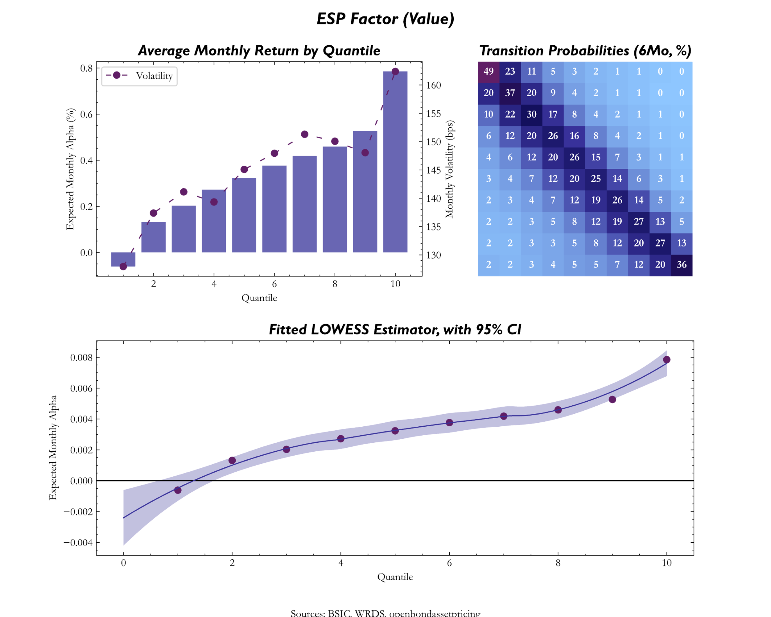
The Value factor aims to target bonds that are “cheaper” (higher spread) relative to other bonds which are deemed to be more “expensive” (lower spread) judged by a specific financial metric. A common characteristic variable used for cross-sectional comparison of credit issuers is the credit rating, which however tend to be backward-looking and lagging indicators of fundamental credit quality. More sophisticated signals for Value in credit investing have been proposed. Frieda and Richardson (2016) used expected default rates and recovery rates to construct a fundamental Value measure, whereas Dor et al (2020) proposed two alternatives, ESP (Excess Spread to Peers), and SPiDER (Spread Per unit of Debt to Earnings Ratio).

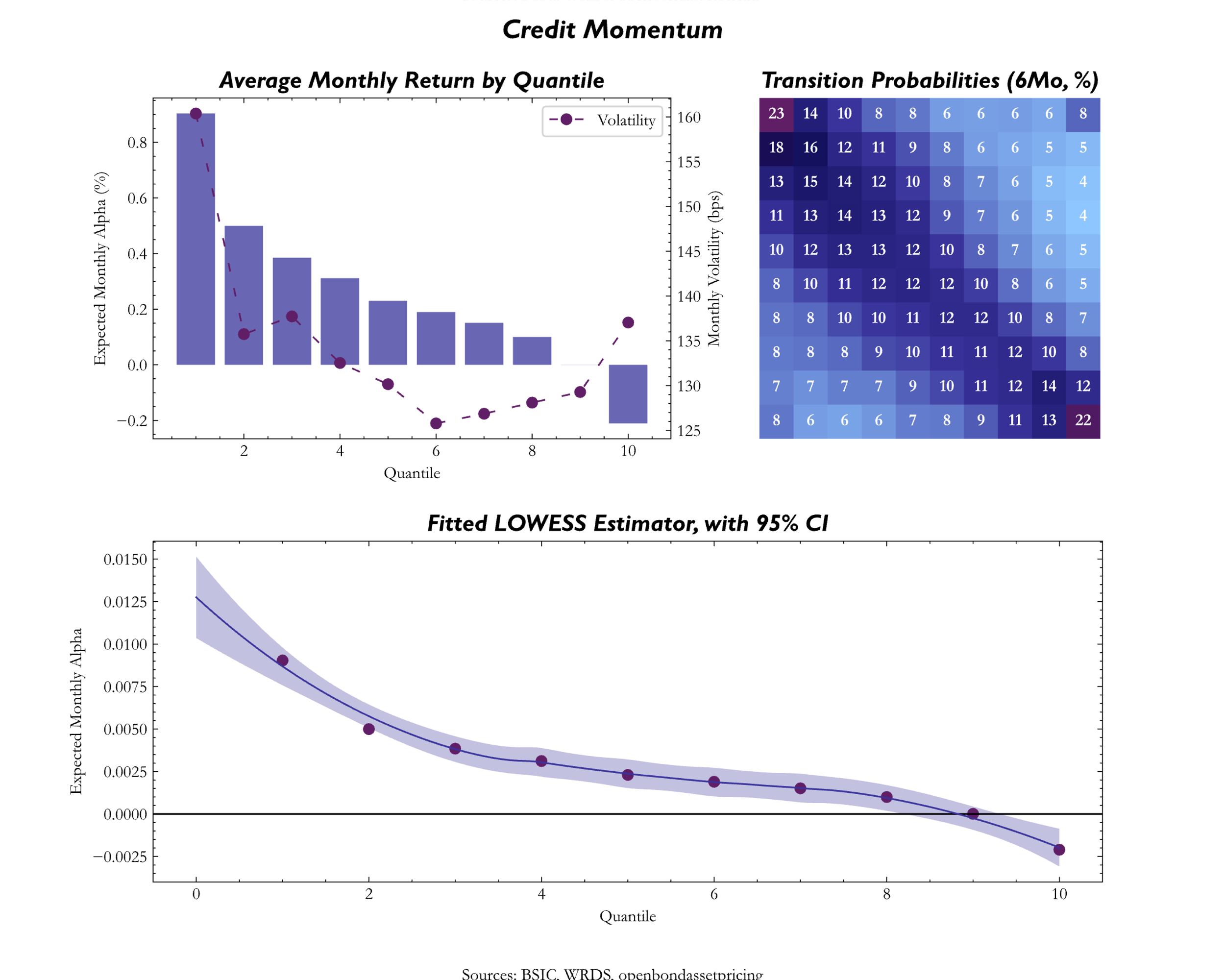
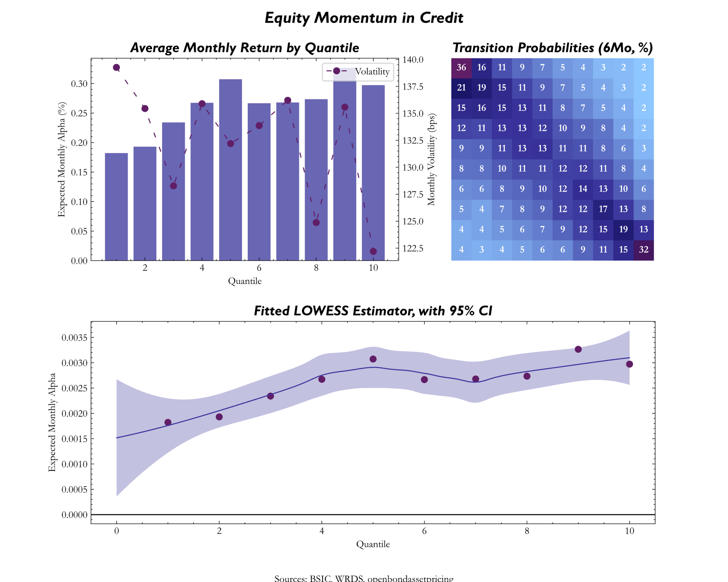
In credit, the Momentum factor seeks to invest in bonds that outperformed in terms of price (credit excess return) over a specified time horizon (e.g., 3, 6, or 12-months). However, it is worth to highlight that bond markets are more price-inefficient than equities due to widely used buy-and-hold approach by investors, thus making bond prices alone insufficiently robust to build a Momentum signal on, especially in the case of IG credit. Moreover, research done by Khang and King (2004) and Gebhardt et al. (2005) found that bonds’ prices display mean reversion, and further analysis by Jostova et al. (2013) indicated minimal effects from following Momentum strategies in IG, but a more meaningful impact when dealing with HY. This finding on Momentum strategies in the HY space was confirmed by Pospisil and Zhang (2010). Instead of relying of bond prices, Dor et al. (2021) proposed a different way to measure Momentum signal in credit, by relying on what they defined as EMC (Equity Momentum in Credit), which uses past equity returns. The basic idea behind EMC is that stock prices tend to react more swiftly and meaningfully to new information and that stock price performance often has a spill-over into bond prices.

The Size factor privileges companies who are smaller in size. In the literature there was not much research on Size as a factor, with only Houweling and Van Zundert (2017), which are suggesting that there is a positive Size premium in credit, whereas Alquist et al. (2018) argued that the Size effect fails to deliver a consistent premium in the case of bonds. Moreover, Dor et al. (2020) found that, when controlling for systematic risk exposures and characteristics, portfolio of small issuers tends to underperform portfolios of large issuers. Overall, there is little evidence that Size is a relevant factor in credit, and that it cannot be exploited by credit investors in the same way as equity investors.

What is Carry? Carry can be defined as the return of an asset assuming that market conditions do not change. For credit investments Carry is represented by the credit spread plus the roll down on the credit curve (Koijen et al., 2018), but Frieda and Richardson (2016) instead used only the credit spread, more specifically the option-adjusted spread (OAS). Such way of representing the Carry signal neglects the roll down, and it works only if the credit curve is flat (i.e., roll down is zero), but if the curve has a positive (negative) slope, OAS will underestimate (overestimate) carry. Since most issuers have positive sloped credit term structures, OAS will tend to underestimate carry, hence it is an imperfect measure of the factor. Nevertheless, the other alternative is to estimate the whole credit curve for every issuer, and such exercise would add extra layers of complexities to the Carry measure, thus the authors argued that OAS strikes a reasonable balance between precision on one hand, and simplicity and transparency on the other.

Quality in the credit space is similar to the Quality factor for equities, with the only difference that metrics for bonds tend to focus on leverage and interest coverage ratios. Henke, Kaufmann, Messow and Fang-Klingler (2020) they built a measure of Quality based on 14 different company-level fundamental variables (i.e., balance sheet variables). All these variables were used to identify high-quality companies, that are those which have good profitability, liquidity and operating efficiency. They find that there is little evidence on the presence Quality premium for IG corporate bonds, although it is beneficial in case of HY.

Low-risk factor, also referred to as Defensive, is often expressed as a sub-set of the Quality factor. Low-risk factor signal target shorter-date, lower rates bonds. In the literature it has been shown that short-dated credit risk consistently outperforms longer-dated spread exposure on a risk-adjusted basis (Ilmanen et al., 2004) and that low-risk assets tend to deliver higher risk-adjusted returns (e.g., Frazzini and Pedersen, 2014). Measures of Low-risk are similar to the ones of Quality factor with the addition of also considering the remaining maturity of the security.

Data

Data gathering for a systematic credit project undoubtedly demands a section of his own: data for credit markets is scarce and, even when it is available, it displays some inconsistencies, or it is incomplete. Hence, one should be very careful in handling such data and continuously assess its soundness. Thus, we took a rigorous approach, coupled with our own qualitative judgement, in order to transform the raw dataset into something that was “tractable” for our analysis.

To begin our research, we considered time series of bond returns, financial ratios of the issuers, and their stock price returns. Data on bond returns were retrieved from openbondassetpricing.com and WRDS, preferring the former, as it contains a few additional adjustments. First of all, data is corrected for Market Microstructure Noise (MMN), which is primarily comprised by bid-ask bias and is strongly time-varying, as explained in Dickerson et al. (2023a); secondly, the maintainers of the dataset fix an issue regarding WRDS capping bond returns at 100%, substituting those datapoints with the figures from BofA, which allows the returns to show their actual values.

The datasets from openbondassetpricing and WRDS have already been processed, in line with the method outlined in Dickerson et al. (2023b).

In order to carry out a robust analysis of the dataset, we perform some further data cleaning on the bond returns database:

We remove bonds with time to maturity higher than 30 years, since this would require additional assumptions about the evolution of the yield curve past the 30-year mark, which are, most of the times, arbitrary,
We fill data which is constant for issues (number of coupons, accruing date, offering date, maturity, first interest date) in the rows where it is missing,
We remove defaulted bonds, as this skews the OAS calculation and would entail calculating a probability of default for the bond, which is outside the scope of the article,
We remove bonds maturing in less than 1 year and Zero-Coupon Bonds
We only keep bonds for which we have at least 36 months of observations, as some of our signals, such as momentum, are based on past returns,

After that, we link each CUSIP to the respective issuer, using the CRSP Link Database from WRDS. The link is far from perfect, and we find that only ~90% of our bond observations are associated with a PERMNO. We use the PERMNO to download financial ratios and equity prices, which will later be used for signals. We also download Short Interest Data from WRDS, since it has been documented as a good proxy sentiment factor, but due to the very scarce availability of the data (we would narrow down our investable universe to only 7%), we decide not to proceed with it.

Then, we proceed with the OAS calculation. Since we removed bonds with embedded optionality, the OAS reduces to the Z-Spread, which is the spread that, added to the discount curve, equals the NPV of the bond to its market price.

$P=\frac{c_1}{1+r_1^f+Z^{mkt}}+\frac{c_2}{\left(1+r_2^f+Z^{mkt}\right)^2}+\ldots+\frac{c_N}{\left(1+r_N^f+Z^{mkt}\right)^N}$

To compute the Z-Spread, we use the QuantLib library, getting the zero-coupon curve data from “Discount Bond Database”, whose research can be found in Filipovic et al. (2022). For the specifics of how we calculated the OAS, and all the variables we used for the analysis, we refer you to the GitHub repository, which is linked at the top of the article. We choose to use QuantLib as it already takes care of considering the correct calendar, settlement days, and day count convention in calculating the cashflow schedule of each bond.

The next step we took to be able to conduct a more granular analysis was dividing the data in buckets. To divide bonds in “buckets”, we carefully evaluated the trade-off between a granular and precise distinction of bonds that have the same drivers, and the fact that we need enough bonds in each bucket at any point in time for our analysis to be robust. Hence, we divided based on three variables: rating, industry, and duration. For rating, we divided bonds between IG and HY, based on the S&P rating number. For Industry, we used the first digit of the SIC Code to divide the bonds into 5 macro-industries groups.

Industry Bucket #1: Agriculture, Forestry, Fishing (0), Mining (1), and Construction (1)
Industry Bucket #2: Manufacturing (2, 3), Wholesale Trade and Retail Trade (5)
Industry Bucket #3: Transportation and Public Utilities (4), Public Administration (9)
Industry Bucket #4: Finance, Insurance, Real Estate (6)
Industry Bucket #5: Services (7, 8)

Although we recognize that, nowadays, NAICS is a more widely accepted classification method for industries, since it takes better consideration of tech companies, our analysis goes back to 2002, when NAICS was not available and SIC Codes were the industry standard. For duration, we partition in 2 quantiles – short and long duration.

Factors Construction

In this section, we outline the methodology used to evaluate our factors. In line with the literature, and as mentioned in the introduction, we evaluate corporate bonds on a relative basis rather than in absolute terms. Therefore, to evaluate the soundness of a signal, we take the following approach: as previously mentioned, we first divide the bonds into buckets for each timestamp, partition our bonds in quantiles based on the signal raw value, and use a measure of “excess returns” (over duration-matched treasuries) to determine the ability of the signal to generate meaningful alpha.

Then, we compute the signal for each bond at each point in time: the methodology to construct it will be outlined for each factor, but overall, the intuition is taking the spread from the “bucket” average at each point in time and divide each group of bonds into quantiles.

To measure the performance of our signal, we choose to use the residual return, as explained in Dor and Florig (2024). First, we computed Duration Times Spread (DTS), a measure of credit volatility of a corporate bond introduced by Dor et al (2007), that is calculated by multiplying the OAS and the Spread Duration together. Then, we proceed to calculate the residual return for a bond $i$ belonging to the bucket $k$ by subtracting systematic return from the unadjusted return:

$r_i^{resid.}=r_i^{unadjusted}-r_i^{systematic}$

where systematic return is calculated as

$r_i^{systematic}=DTS_i^{rel.}\times{\bar{r}}_k$

The term ${\bar{r}}_k$ represent the weighted average returns of all bonds belonging to the bucket $k$ , whereas $DTS_i^{rel.}$ is the relative DTS of the bond, computed as DTS over the weighted average DTS of the bonds in bucket $i$

$DTS_i^{rel.}=\frac{DTS_i}{{\bar{DTS}}_k}$

Although the original paper uses the weighted average for ${\bar{r}}_k$ and $\bar{DTS}}_k$ , we opt to use the weighted median instead. This choice is justified by the fact that our dataset contains several outliers, which would have undesirable effects on the mean; thus, we choose the weighted median as a more robust proxy for each bucket.

We now present how we computed the factors and present, for each of them the value of the signal for each quantile to show how exposures to different percentiles of the factor yield different performance measures. For each factor, we show a plot representing the expected alpha by and the interpolation obtained through LOWESS (LOcally WEighted Scatterplot Smoothing) using scikit-misc.

Furthermore, we also plot the transition matrix for each bucket. Analyzing it is important, especially when designing a strategy for credit, where we want to limit as much as possible our turnover: we should prefer signals for which bonds tend to stay in the same quantiles, since, otherwise, we would be forced to either rebalance our portfolio too often or hold on to bonds even when they leave our “target” quantiles.

For Carry, we used the values of the OAS, as presented by Frieda and Richardson (2016) and divided correspondingly in quantiles for each point in time.

For Momentum we used two different measures, that lead to different conclusions: the values of the (monthly) credit excess returns, as defined by Frieda and Richardson (2016) where

$CER_t=\frac{1}{12}OAS_{t-1}-\mathrm{Spread\ }{\mathrm{duration}}_{t-1}\times\left(OAS_t-OAS_{t-1}\right)$

and Equity Momentum in Credit where we just included the rolling 6 and 12-month returns for the corresponding stock. For both credit and equity momentum we then included only the 12-month momentum as the signal was more consistent than the 6-month momentum. We see from the chart that the 2 metrics lead to different performance across quantiles, where the CER measure actually looks like a reversal where top quantiles tend to have lower expected signal compared to bottom quantiles, while equity momentum tends to act as the other factors.

For the value factor we used the excess spread over peers, as the value of difference between the single bond’s OAS and the average OAS of its bucket $k$

$ESP_i=OAS_i-{\bar{OAS}}_k$

Then, we ran an OLS regression at each point in time and for every bucket $k$ all the $ESP_i$ metric of the bonds belonging to such bucket on a constant and 3 company’s fundamentals: Debt/EBITDA, Interest coverage ratio and Debt/Equity ratio.

$ESP_{i,t}=b_0+b_1Debt/EBITDA_{i,t}+b_2Interest\ coverage\ ratio_{i,t}+b_3Debt/Equity_{i,t}+\varepsilon_{i,t}$

We stored the residuals $\varepsilon_{i,t}$ from the OLS, which was then used to compute the quantiles and the expected alphas.

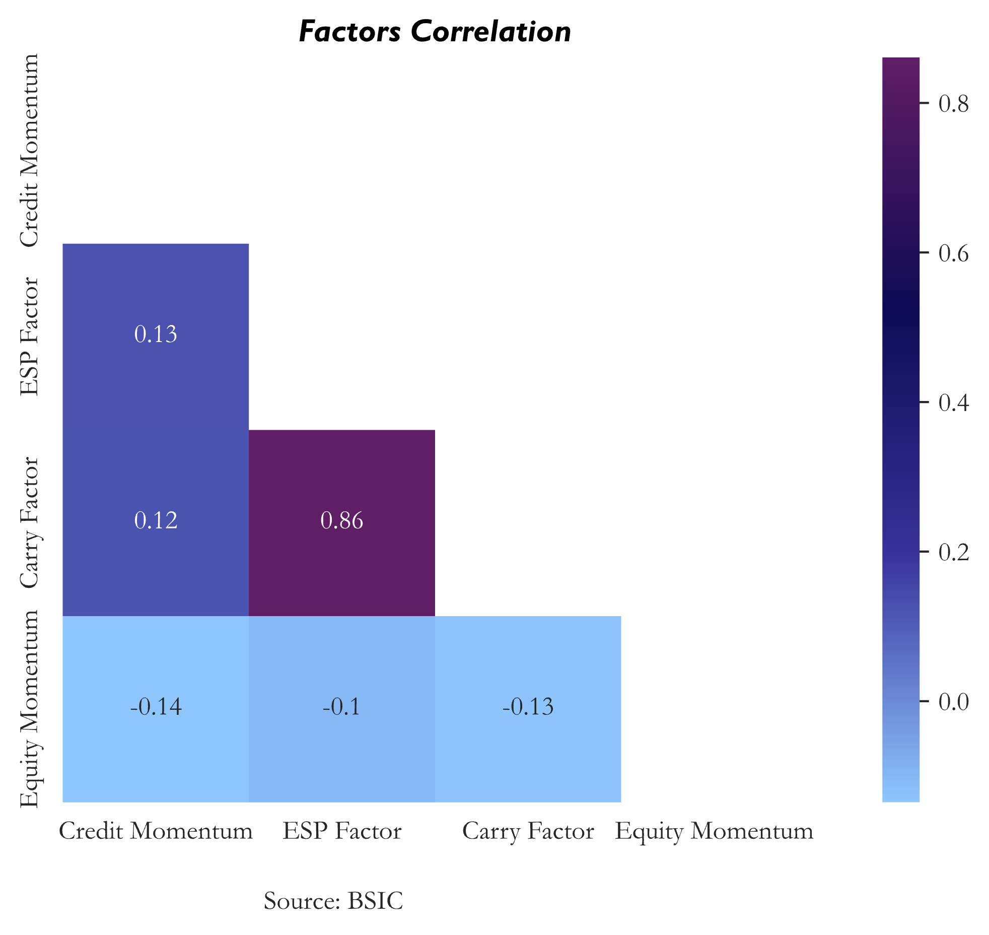
The factors are overall little correlated with the exception of Value (Excess Spread to Peers) and Carry (OAS), which are correlated by construction.

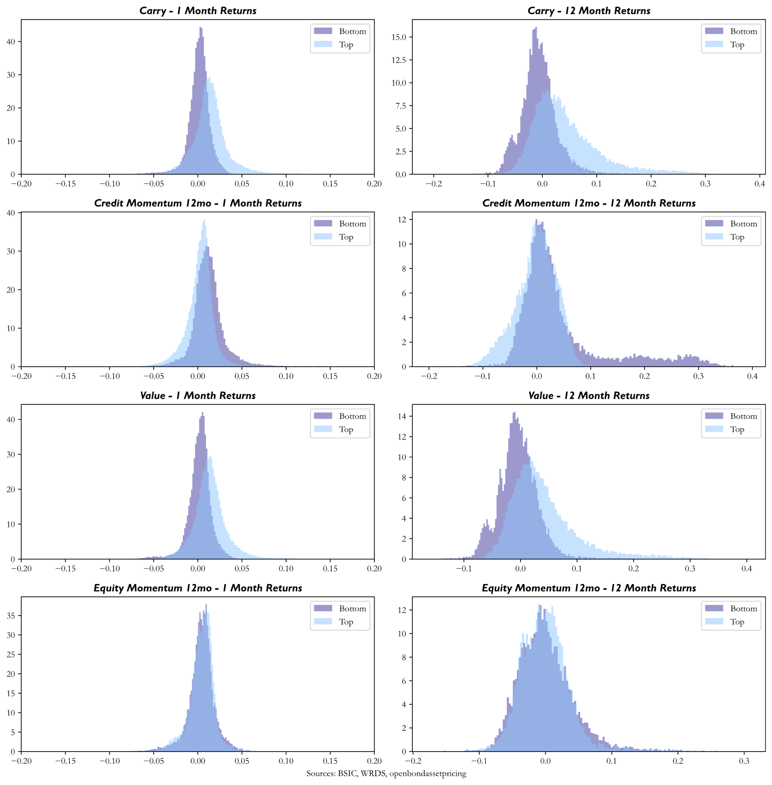
Furthermore, for each factor we aim the show the effects of excessive concentration in bottom quantiles versus top quantiles. To this end, as proposed by Dor and Florig (2024) we simulate at each point in time 1000 portfolios containing 10 bonds in the last decile and 10 in the top decile and plot the simulated distributions. For each factor, we show the distribution of 1-month and 12-month returns of the simulated portfolios, highlighting the impacts that concentration can have. The logic of this simulation is that real portfolios in credit will never be as diversified and furthermore, due to illiquidity, it might be hard to get out of bottom-quantile bonds.

Strategy Overview

To construct our trading strategy, we follow the approach presented in Dor and Forig (2024): the first step is understanding why we are using signals, and not directly portfolios to drive our trading decisions. Directly using portfolios for computing the signals is an intuitive way to approach the problem. However, introducing traded portfolios as signals introduces the problem of how to construct such portfolios and can induce to excessive trading and therefore transaction costs. Therefore, as in the paper, we compute a single composite signal that is just a linear combination of the different signals

$\alpha=\sum{w_if_i\left(x_i\right)}$

where $w_i$ is the weight associated with signal $i$ , and $f_i\left(\cdot\right)$ is the mapping associated with signal $x_i$ .

To isolate each security’s idiosyncratic return, we use the bond’s residual return, as presented in the previous section. The residual return will therefore be our signal, (we plotted the values of the expected alpha for each factor in the previous section); as a last step, we demean and standardize the signals to make them comparable. The next step is selecting the factor weights: to achieve this, we use partial returns, which are given by the coefficients of a time series of cross-sectional regression of residual returns on all the signals, similar to a Fama-Macbeth procedure. This makes it easier to understand how they can be used as weights, as they are indeed the coefficients of a linear combination of signals that maximizes the correlation between residual returns and alpha. Furthermore, they can be interpreted as the “returns” of a factor mimicking portfolio.

As it has been shown in Dor and Florig (2024), partial returns display signs of autocorrelation: we therefore implement a simple trend-following model for our weights, leaving a formation period at the beginning of our investment where the weights $w_t$ evolve in the following manner

$w_t=\left(1-\alpha\right)w_{t-1}+\alpha\frac{r_t}{v_t}$

where $\alpha$ is the smoothing parameter, $r_t$ is the partial return, whereas $v_t$ is the partial return volatility, computed as a weighted average of the squared partial return and the previous estimate of volatility

$v_t=\left(1-\alpha\right)v_{t-1}+\alpha r_t^2$

The model is parametrized according to the half-life of $\alpha$ which essentially represents the time of decay and frequency of updating.

Finally, given the composite signal weighted accordingly, for each date we sort the cross-section of bonds and trade the 25 bonds with the highest signal value, according to an equally weighted portfolio.

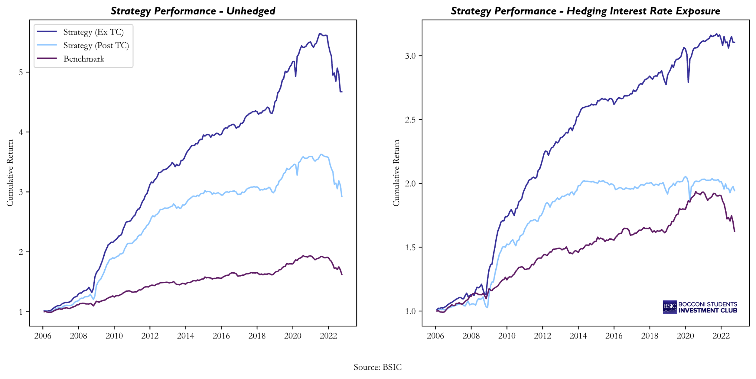
We now show the resulting equity curve and the main summary statistics of the implemented strategy, comparing it with the equal-weight index and with the strategy assuming a fixed level of transaction costs multiplied by the number of bonds traded each month.

Overall, the strategy performed very well in the early 2010s, reaching a rolling Sharpe Ratio of more than 5 around 2012 and obtaining an overall Sharpe Ratio of 2.54 over the whole period. Of course, this is a simple and rather naïve implementation of the strategy, transaction costs could and should be modelled in a more robust manner to account for the time-dependence of bid-ask spreads and for the illiquidity of some positions. Furthermore, in future research, turnover limits could be implemented by closing positions only if bonds go below a certain quantile threshold by implementing the transition probabilities shown in the previous section. In addition, data are missing in many dates and volatility may therefore be understated and there might be survivorship bias inherent to the dataset and our decision to exclude defaulted bonds. This article seeks, however, to present to the reader a structured approach to systematic credit investing by explaining the process in simple steps from start to finish; with future research and additional resources the final strategy may be refined to bring to even better results.

References

[1] “What drives credit? Understanding the cross section of expected corporate bond returns”, Markets Division, Bocconi Students Investment Club, 2022

[2] Alquist R., Israel R. and Moskowitz T., “Fact, Fiction, and the Size Effect”, 2018

[3] Dickerson A., Robotti C., and Rossetti G., “Return-based anomalies in corporate bonds: Are they there?”, 2023a

[4] Dickerson A., Robotti C., and Rossetti G., “TRACE (WRDS) Data README”, 2023b

[5] Dor B. et al., “DTS (Duration Times Spread)”, 2007

[6] Dor B. et al., “Systematic Investing in Credit”, John Wiley & Sons, 2020

[7] Dor B. and Florig S., “Integrating Multiple Signals in Systematic Corporate Bond Selection Strategies”, 2024

[8] Filipovic D. et al., “Stripping the Discount Curve – a Robust Machine Learning Approach”, 2022

[9] Frieda A. and Richardson S., “Systematic Credit Investing”, AQR Capital Management, 2016

[10] Gebhardt R. W., Soeren H., and Bhaskaran S., “The cross-section of expected corporate bond returns: Betas or characteristics?”, Journal of Financial Economics, 2005

[11] Henke, H. et al., “Factor Investing in Credit”, The Journal of Index Investing, 2020

[12] Houweling P. and Van Zundert J., “Factor Investing in the Corporate Bond Market”, 2017

[13] Ilmanen, A. et al., “Which Risks have been best Rewarded?”, Journal of Portfolio Management, 2004

[14] Israel R., Palhares D., and Richardson S., “Common factors in corporate bond returns”, AQR Capital Management, 2017

[15] Jostova G. et al., “Momentum in Corporate Bond Returns”, The Review of Financial Studies, 2013

[16] Kamenski P. and Lam R., “Factors in Quant Credit”, Man Numeric, 2021

[17] Khang K. and King T., “Return reversals in the bond market: Evidence and causes”, Journal of Banking & Finance, 2004

[18] Koijen, R. S. et al., “Carry”, Journal of Financial Economics, 2018

[19] Pospisil L. and Zhang J., “Momentum and reversal effects in corporate bond prices and credit cycles”, The Journal of Fixed Income, 2010

[20] Preston A. et al, “Quantitative Credit: Alpha Opportunities for Early Mover”, Man Group, 2021

Published by BSIC on 5 May 20245 May 2024

0 Comments

Leave a Reply Cancel reply

Corporate Finance Markets

Exploring the Practicality of Merger Arbitragе

Markets

Market Recap 05/05/2024

Markets

The Copper Paradox

A Systematic Approach to Credit Investing

Published by BSIC on 5 May 20245 May 2024

0 Comments

Leave a Reply Cancel reply

Related Posts

Corporate Finance Markets

Exploring the Practicality of Merger Arbitragе

Markets

Market Recap 05/05/2024

Markets

The Copper Paradox