Backtesting Series – Episode 1: Introduction

Download PDF

Introduction

In this article, we present the first episode of a series on backtesting. We want to provide the reader with an immersive analysis of this powerful tool and analyze all the processes that lead to its optimization and implementation. The series will consist of the following parts:

• Part 1: Introduction
• Part 2: Cross-Validation techniques
• Part 3: Portfolio Construction & Portfolio Optimization, Factor Models
• Part 4: Backtest Analysis – Metrics, Drawdown Analysis
• Part 5: Introducing TCs, assessing capacity, preparing for production

In this episode, we are going to set the scene for the whole series, giving an overview of how a backtesting pipeline should look like, and give a thorough overview of the Sharpe Ratio, Information Ratio, and Information Coefficient. We are going to cover the non-trivial question of using normal returns vs log-returns and, finally, we are going to explain how we generated the data that we will use to test the robustness of the techniques we will propose in the upcoming episodes.

We will start from the basics by defining alpha. That is a measure of investment performance, most used to describe returns that exceed the market or a benchmark index. For active management funds, generating alpha is a primary objective and shows the value added by a portfolio manager or a strategy above what could be gained just by following the market or other factors.

In the development of a trading strategy, the goal is to design a model that delivers indicators, called alpha signals, that are predictive of excess returns and use them to construct a portfolio. Alpha models are automated and predictive. They describe, or decode, some market relation and are designed to have some edge, which allows traders to anticipate the future with enough accuracy that, after allowing for being wrong at least sometimes and for the cost of trading, allow them to still make money. An alpha contains rules for converting input data to positions or trades to be executed in the financial markets.

Data and Look-ahead biases

The starting point for every strategy is the data. The process of obtaining high-quality data and checking for potential problems is a tedious one but is also the necessary condition for a robust alpha model. We won’t go into data cleaning in this series, and we will assume that the data has been checked for correctness. What we want to spend some time on, however, are the biases that can occur during the research process and can undermine the statistical robustness of the backtest.

One of the most common biases that can occur when building an alpha model is look-ahead bias. That happens when you allow future information to influence decisions that are meant to be made only using current or past data. An incorrect time labelling, for example, can lead to a look-ahead, or a research bug of inadvertently using future data. In contrast, real-time production trading is free of such issues, since it is based only on data available up to the current moment without access to any future data. Researchers using machine learning techniques also can introduce lookahead bias. They may tune some hyper-parameters on the entire data sample and then use those parameters in the backtest. Hyper-parameters should always be tuned using only backward-looking data looking for a correct Train-Test splitting. Similarly, in the area of sentiment analysis, researchers should take note of vendor-supplied sentiment dictionaries that may have been trained on forward-looking data. Just like in backtesting, that can result in an overly optimistic or skewed sentiment classification because the dictionary has been informed by future events that shouldn’t have been available at the time.

A more subtle source of lookahead bias can affect large quantitative portfolios that rely on the same forecasts over extended periods. Past trades done for this type of portfolios affect prices by market impact, making the forecast performance look better via a self-fulfilling prophecy. Indeed, if you later backtest a trading strategy on the same period, the results may be skewed. It is a consequence of past trades that have already influenced the prices, making it easier for the model to predict price changes. This creates a self-fulfilling prophecy where the model looks as if it’s performing well, but in reality, it’s mostly because your trades impacted the prices in your favor.

Moreover, correct lifespan information is important also for avoiding survival bias, a fallacy of running quant research on assets alive today but ignoring those no longer active magine you’re testing a trading strategy that invests in S&P 500 stocks. It’s important to note that the composition of the S&P 500 today is not the same as it was 10, 20, or 30 years ago. Companies are added or removed from the index over time due to changes in performance, market capitalization, mergers, acquisitions, or bankruptcies. Now, if you backtest your strategy using only the companies that are currently in the S&P 500, you’re testing how today’s survivors would have performed over the past few decades. This approach ignores companies that were part of the S&P 500 in earlier years, such as those listed in 2000 but have since been removed due to poor performance or bankruptcy. By doing this, you’re effectively excluding the “failures,” leading to an unrealistic assessment of your strategy’s historical performance. Remedies for this issue can be implementing an objective methodology for inclusion that can be implemented at any time or specifying a robust rule in the backtesting process for the event of a delisting.

Another major issue that can occur while working with your dataset is called data snooping. It refers to the practice of extensively testing multiple strategies on the same dataset without a proper prior until you find one that appears to perform well. However, the strategy’s apparent success is often due to chance rather than a real, generalizable pattern. Data snooping can lead to misleading conclusions and overfitting, where a model or strategy seems to perform well in historical tests but fails to work on new, unseen data. In other words with data snooping your historical test set isn’t any more an actual test set and your statistical significance or p-values are not relevant any more.

Defining the investment universe

An important step in developing an alpha model is choosing the target set of assets to be traded, this set of assets is called the investment universe. It is possible to restrict it along one or more dimensions such as asset class, geography, industry or individual instruments. The universe choice is typically driven by the coverage of the input data or the idea that is behind the alpha model, although signals can be designed and tuned specifically for a certain universe even if the data has wider coverage.

Linear vs Log Returns

We think it’s important, first of all, to define returns and their statistical properties. The question of whether returns are Gaussian is an empirical one. We all know assuming cross-sectionally gaussian returns is an approximation (a significant one, even) – we usually do it to make the analysis more tractable, and our returns better-behaved statistically. However, this still does not make them easily tractable in time series analysis. We first define linear returns for a security as:

Where and denote the price of the security at time and while is a factor that adjusts for possible dividends or other sources of income. Also, linear returns are the ones that define the daily portfolio PnL through the dollar position :

On the other hand, we define log returns as:

But why would we want to use log-returns, which are just a first-degree approximation? Even if we were to assume linear returns to be normally distributed, the cumulative total return is not normally distributed, and its distribution rapidly diverges from the normal distribution. Instead, log returns are additive over compounding. This implies that the log of the compound return is equal to the sum of the log returns in the same period, and if the log return is normal, so is the log of the compound returns. Moreover, if the returns are independent, the variance of the log of compound log return is equal to the sum of the variances. We define compounded net returns over time with the following common approximation:

Over short-term horizon, where asset’s returns are usually of order 1%, we can approximate the difference between log and linear returns as follows:

This delivers a difference between linear and log returns that is of order . Said that, going back to compounded returns, this allows us to make an even further approximation for short-term horizon:

Remark that is always important to verify the accuracy of this approximation and that can vary between different asset classes. For example, when the assets are equities, the approximation is usually considered adequate for daily interval measurements or shorter.

The different statistical properties between linear and log returns affect forecasting especially over longer horizons, because the operators of (linear) expectation and (concave) log do not commute. Though the statistical distribution of log returns may have better mathematical properties than those of linear returns. Still, it is the linear return-based PnL that is the target of portfolio optimization. It is although of common practice to construct a model on log returns, benefitting of their statistical properties, and then backtest it with linear returns.

To prove what we have explained above, we drew returns from an i.i.d. normal distribution centered at 0 and with std . After computing linear compounded returns and log compounded returns this are the results we obtained:

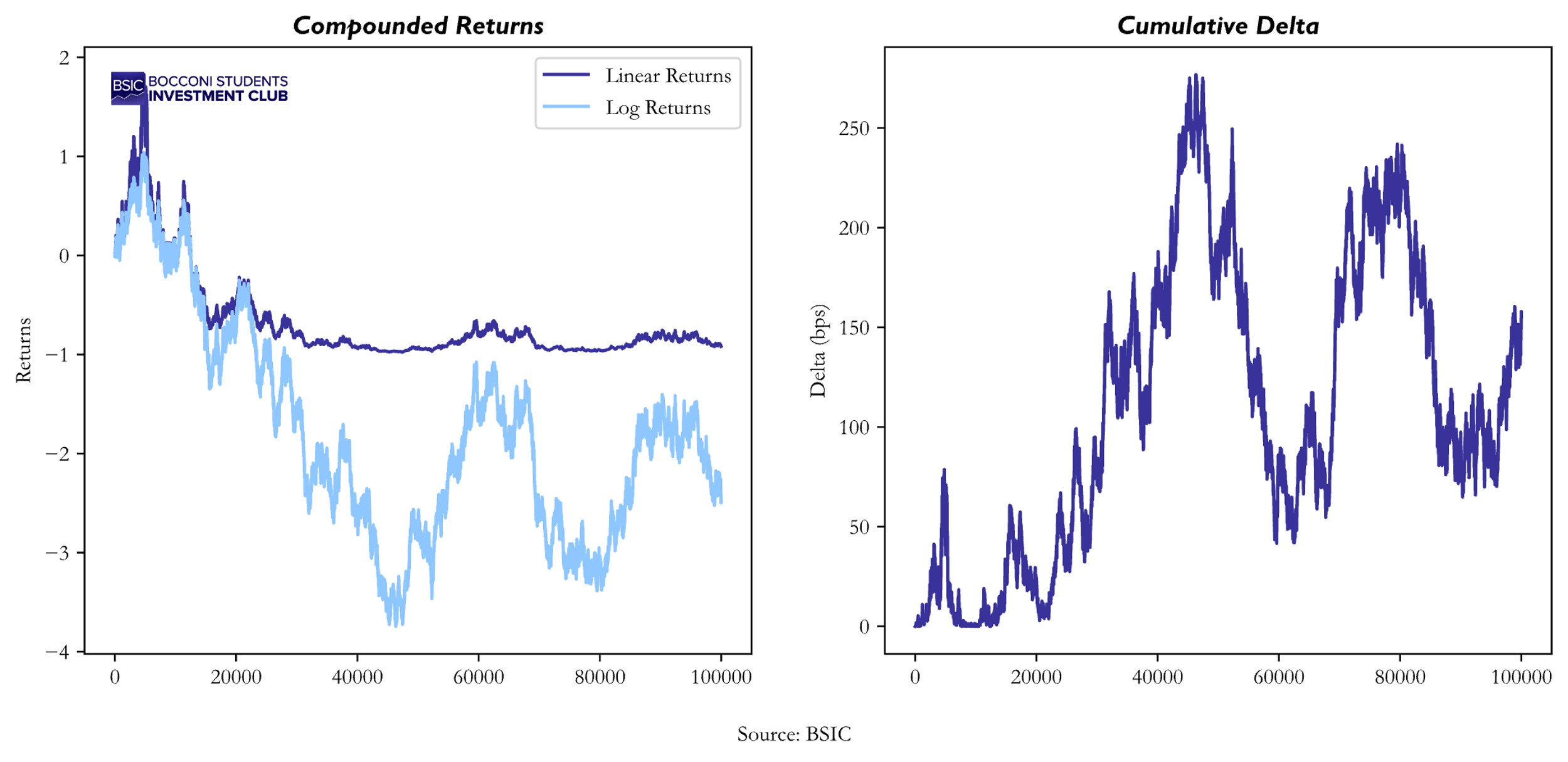
From the graph above appears that our approximation for compounded linear and log returns can hold for short period of time but after a while, they begin to diverge. Indeed, at the end of the process, the delta between the two of them reaches 156.6bps after it have reached spikes of 250+bps. But let’s have a closer look to the distribution of monthly compounded returns to better understand the statistical properties of log and linear returns.

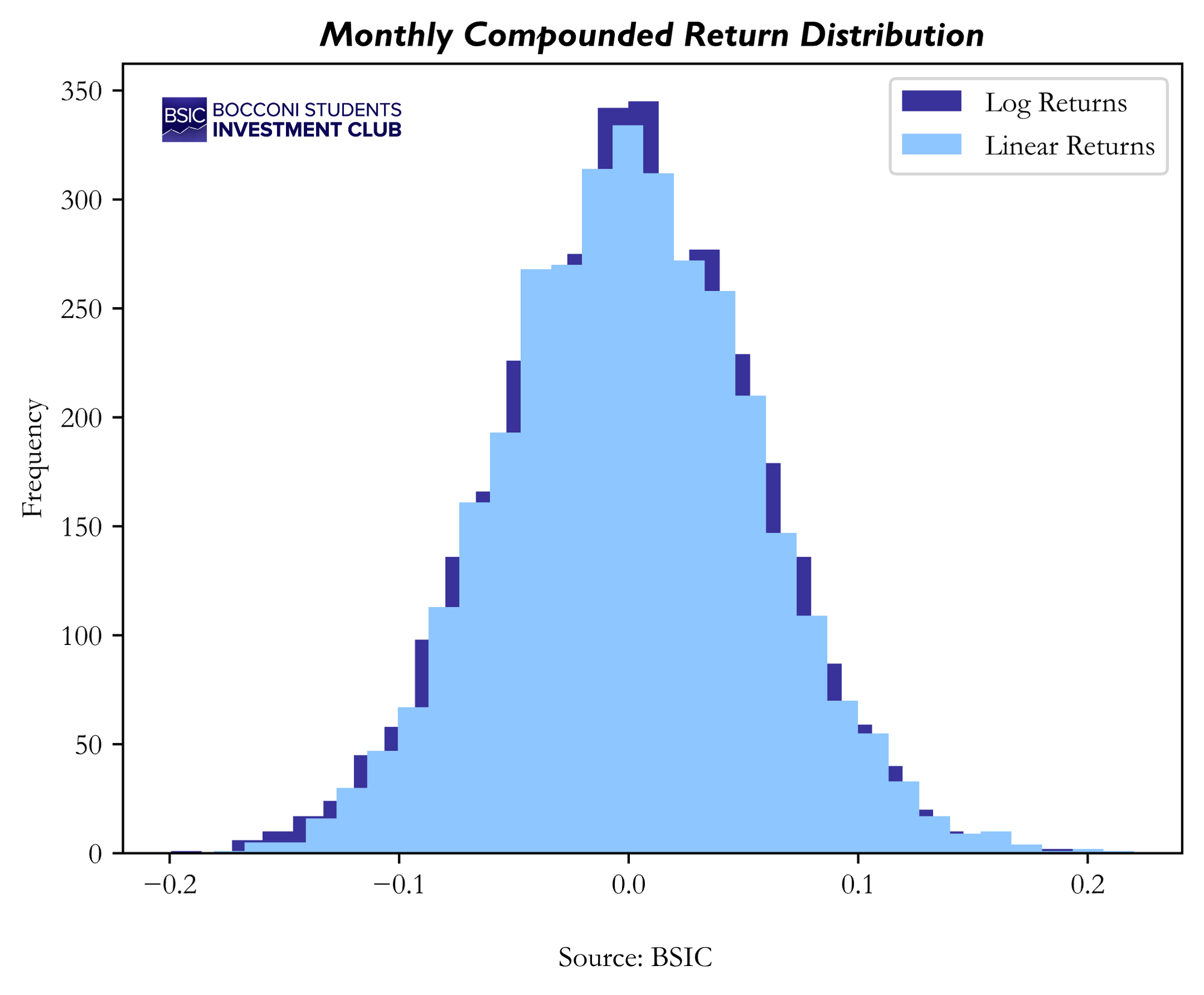
Since these plots are probably not enough explicable at first sight, we extended our analysis to better understand the change in normality between log and linear returns. We applied D’Agostino and Pearson’s test, which combines skewness and kurtosis into an omnibus test of normality. The results revealed a p-value of 0.013 for the linear returns distribution, which is below the 0.05 significance threshold. This allows us to reject the null hypothesis of normality for the linear compounded monthly returns distribution. In contrast, the p-value for the log returns distribution increased to 0.441, indicating a significant improvement in normality. This aligns with the statistical properties of log returns we previously discussed.

Portfolio Optimization & Factor Models

Once you have your alpha signals for your universe of assets, you need a way to combine these signals together in an efficient way. This is the step of portfolio construction and optimization, which we are going to elaborate further on in an upcoming episode.

The most popular method is Mean Variance Optimization (MVO), where you maximize the expected return of your portfolio while minimizing the total variance. MVO has its own set of problems, namely that it can lead to sparse solutions (overweight on a handful of assets) and that it can perform very poorly out-of-sample. However, this should not necessarily be traced to a problem with the model itself – often, it is more of a problem with the two inputs: your expected returns and the covariance of the assets. Most importantly, estimation errors in the covariance matrix can be one of the main factors leading to poor performance of MVO. We are not going to elaborate on covariance estimation methods here, but one of the main methods is constructing a factor model, which allows for a more robust estimation of the covariance matrix between assets. Factor models are a great tool, which can be helpful in portfolio construction/optimization, performance attribution, and risk management – we will have a dedicated episode of the series on factor models.

Backtesting Practice

After constructing your strategy and optimizing your portfolios, it is time to evaluate it and backtest it on available data. We will introduce some of the most common practices that exist to do that but we will delve deep into this argument in a following episode.

The most common evaluation scheme you can use is Cross-Validation. The available data is split into a training dataset and a holdout dataset. We will explore two different types of Cross-Validation. The first one is the so called K-Fold methodology. It involves splitting the dataset into K equally sized subsets, or “folds”. For each fold the model is trained on the remaining K – 1 folds and validated on the remaining one. This process is repeated K times with each fold being used exactly once for the validation. In the end, the performance metrics are averaged to provide a more robust estimate of the model’s generalization ability. On the other hand, the second technique we will analyze is the Walk-Forward one. This is particularly used to work with time-series data. The dataset is split based on time. We use historical data up to time and target returns at time . This process is repeated expanding the training window forward in time, while the validation window moves step-by-step through the data.

Moreover, in the episode to come, we will confront these common evaluation schemes to a new methodology proposed by Giuseppe Paleologo (2024) called Rademacher Antiserum. Using Rademacher Complexity it measures the ability of a set of strategies to avoid overfitting by quantifying how much they covary with random noise. By comparing strategies against random noise, this method helps ensure that the chosen model generalizes well to unseen data, thus providing robust backtesting results​. This technique is also able to deliver lower bounds to Information Ratio and Information Coefficient and differently from Cross-Validation, it uses all the data available at the same time, for all the strategies.

The Sharpe Ratio

In the following two paragraphs, we will introduce you to the main evaluation metrics we will use throughout the series, starting from the Sharpe Ratio, the most common measure of the performance of an investment strategy. Informally, the Sharpe ratio can be defined as the risk-adjusted expected excess return of a portfolio with respect to the risk-free rate over the standard deviation of this same excess return:

Where is the sample mean of excess returns and is the sample standard deviation. This basic estimator of the Sharpe Ratio is closely related to the Student’s t-statistic for testing whether a random variable, in this case the returns, is significantly different from zero. The t-statistic is the Sharpe Ratio scaled by the square root of the number of trading periods :

A key problem of the estimator for the SR is that it is biased, meaning that its expected value is not equal to the true Sharpe Ratio . Indeed, the expected value of the basic Sharpe estimator is greater than the true Sharpe Ratio resulting in overestimating . Below is the relationship that links unbiased and biased Sharpe Ratio:

It is possible to define the Bias Factor in relation to the number of trading periods as follows:

Where is the Gamma Function. Consult Mattia Rondato (2018) for a more in-depth analysis of the bias factor and the relationship between the expected value of and .

It is important to note that as the sample size increases, the bias factor approaches 1, so bias becomes smaller with more data. Also, a greater sample size reduces the variance of our basic estimator. On the other hand, variance increases as True Sharpe grows larger. Assuming normally distributed i.i.d excess returns, it is possible to derive confidence intervals for . We present two ways of doing that. The first one uses asymptotic normality, meaning that for large the distribution of the basic Sharpe ratio estimator becomes approximately normal by the Central Limit Theorem. The asymptotic confidence interval is:

Where is the point of estimate of the true Sharpe, is the standard normal quantile corresponding to the desired confidence level (e.g., 1.96 for 95% confidence) and is the standard error computed as . A more robust method to estimate confidence intervals is using bootstrap, where samples are drawn from the original data to compute a distribution for the Sharpe ratio estimator. This method corrects for potential non-normality in the data, although is much more computationally expensive. It involves defining for each bootstrap sample a “studentized” statistic where and are the estimate of the Sharpe and the standard error of the bootstrap. Then after sorting the results in ascending order is possible to form an empirical distribution of the studentized statistic which will be used to define the confidence intervals as follows:

Here and represent the critical values from the sorted bootstrap studentized statistics while and are still respectively the point of estimate of the true Sharpe and the standard error from the whole sample. To give a more comprehensive picture we decided to provide an empirical example of how these intervals actually behave. We simulated normally distributed excess returns from 1000 different strategies, each time implying different values of True Sharpe. Then we computed the asymptotic confidence intervals on rolling Basic Estimator over different window sizes. Due to computational reasons, we did not repeat the same test also for the bootstrap method. Averaging the results from all the 1000 strategies this is what we got:

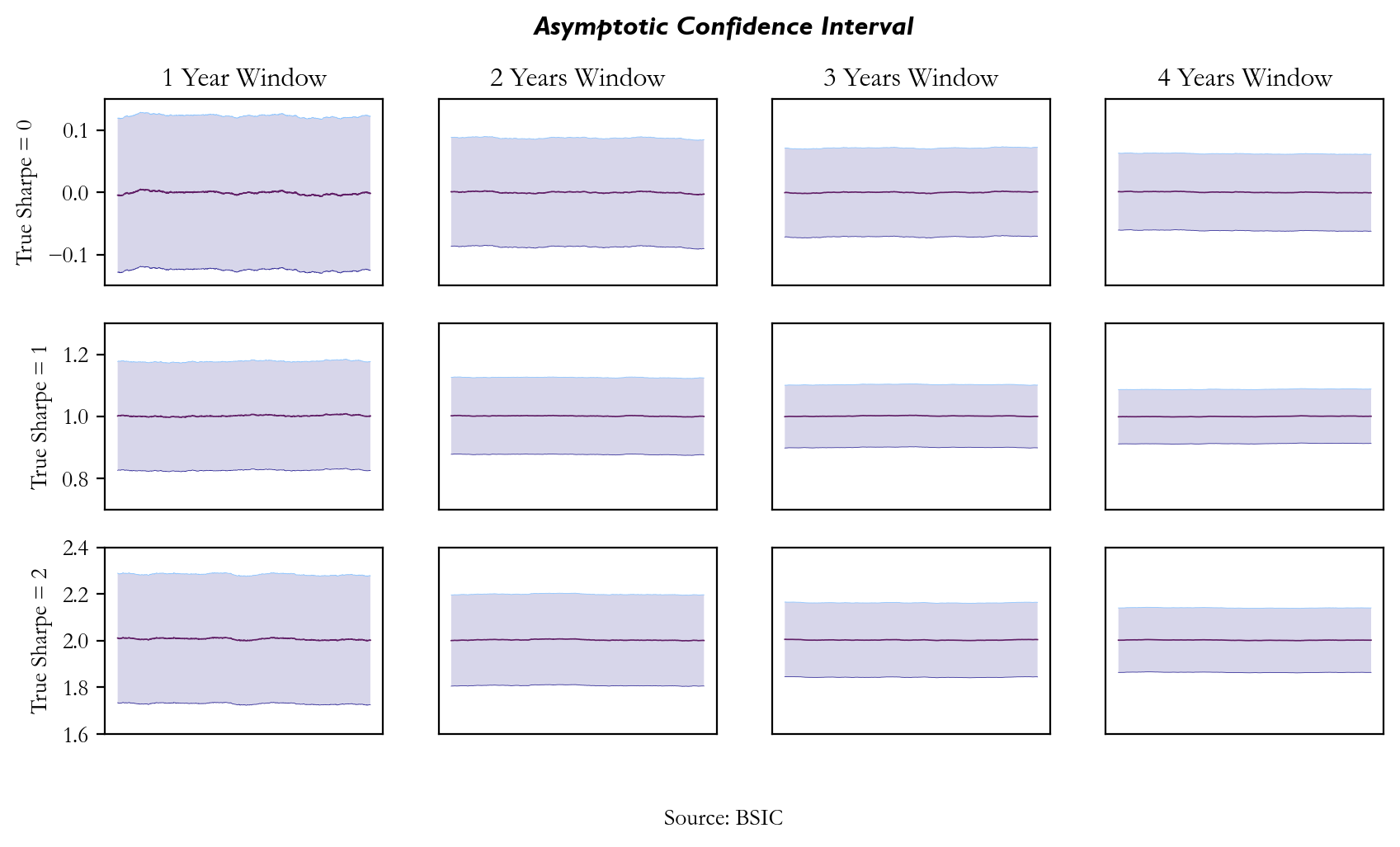
The empirical results over the asymptotic confidence intervals confirm our prior assumptions on the bias factor of It appears clear that as the window size gets larger, the confidence interval gets narrower meaning the bias factor is reduced. Also, by looking at the y-axes range, it is possible to confirm that as True Sharpe grows larger, the variance of our Basic Estimator increases. We repeated the same process over the same sample of randomly generated data, although this time we drew them from a T-Student distribution accounting for more heavy-tailed returns. Here are the results:

We can see that as soon as the normality assumption of excess returns is relaxed, and the in-sample distribution of Sharpe ratios does not converge to normal and moves from mean 0, the results tend to be more inconsistent. Indeed, The asymptotic confidence interval is based on the assumption that the sampling distribution of the estimator (e.g. the Sharpe ratio) approaches normality as the sample size increases allowing for the use of normal-based confidence interval. Using a more heavy-tailed distribution causes underestimation in the true variability of the estimator, especially in smaller windows and wider confidence intervals for small sample sizes, as the asymptotic normality assumption doesn’t hold as well for heavy-tailed distributions. Moreover, it becomes clear how the Basic Estimator that we usually use as performance metric can either underestimate or overestimate the True Sharpe Ratio.

Our personal take is that if you should take anything out of this, it is that you should be pessimistic about your Sharpes. Furthermore, once you have a decently high Sharpe, the estimation error makes it much more worth it to move your attention to other metrics of your strategy; first of all, controlling drawdowns. Sharpe should be your main priority only when you don’t have it.

Information Ratio and Information Coefficient

The information ratio (IR) and information coefficient (IC) are two other metrics that can be used to evaluate the performance of our alpha signals. In this section, we are going to give an overview of these two measures, connect them to the Sharpe Ratio and our predictive model, and give some useful heuristics regarding what you can expect when running a backtest on real data. We’ll move in steps, from a more intuitive definition, to a more rigorous one, and to a proper mathematical definition of these two measures.

First of all, in simple terms, the IR can be seen as a generalization of the Sharpe Ratio; as we will see below, setting our benchmark as the cash portfolio (thus earning the risk-free rate) makes the IR equivalent to the SR. The IC, on the other hand, is a more direct measure of the predicting power of our alpha signal.

Before giving a more rigorous definition of IR and IC, we must briefly introduce the concepts of residual returns/alphas (we will use these two terms interchangeably). Alpha is a rather loose term; the most general definition is that alpha is any excess return over the return of a reference instrument. To give a mathematical “form” to this excess return, we need to decompose the PnL of our portfolio in two parts – the one explained by the benchmark, and the one orthogonal to it. A linear regression is the easiest way to do it – but even then, we can distinguish 3 main types of alphas, which differ in what we consider as our reference instrument.

For the benchmark alpha, we choose the index we are tracking as our reference instrument (e.g. Russell 2000); for the CAPM alpha, we use the market portfolio; for the multifactor alpha, we include all the relevant factors, which will also include the market factor, consistent with what you would do in a factor model.

There are a few conceptual differences in the 3 methods. The benchmark alpha is more relevant to active portfolio managers that track an index; however, the apparent outperformance (alpha) of a PM might just be due to the fact that he chose a bad benchmark. The CAPM alpha solves that, by setting the benchmark as the market portfolio. The multifactor alpha controls for factor exposures, which makes it for a “truer” estimate of PM skill, and for a purer estimate of idiosyncratic returns. That is because if we exclude factors from the regression, it might very well be that the excess returns of the PM were not pure “alpha” but came from harvesting factor risk premia – which is not necessarily a bad thing, but it’s something that is arguably easier than being able to predict “true” idiosyncratic returns, orthogonal to known risk factors. A fair critic to this might be that your idiosyncratic returns are just factors you haven’t discovered yet – which we don’t necessarily disagree with. Regardless of what alpha measure I choose, I would expect my PM to have a positive, statistically significant alpha.

We now have the necessary ingredients to introduce the Information Ratio: using the results from the previous paragraph, the IR is defined as the expected annual residual return over the volatility of the residual return:

From this, we can easily derive that if we assume our benchmark to be the cash portfolio, thus earning the risk-free rate, our Information Ratio will be

It is important to make a distinction between the ex-ante IR and ex-post IR. When running a backtest, we are in the dream world of the ex-ante IR. We can see the ex-ante IR as the maximum IR we can get ex-post – that is, if we squeeze all the information out of our signal when we implement our portfolio. We can repeat the same reasoning for the SR. If our portfolio construction/optimization process is sub-optimal, our realized IR will be lower than the in-sample one. The delta between the two has a specific name: Information Loss (IL).

Moving on the IC – the information coefficient is the correlation between our alpha signals and the returns of our asset. There is a very useful rule of thumb relating the IC to the IR, which is called the fundamental law of active management, which says

Where breadth is the number of independent predictions we make. This should be taken more as a diagnostic measure rather than being used for portfolio construction, and basically says that we can improve our IR either by improving our model (IC) or by expanding our asset universe or how often we make predictions (the breadth). If we can improve one of the two without sacrificing the other, we should always do so. An interesting empirical question would be which one of the two is easier to improve: our intuitive take is that it is easier to find a high conviction signal that works for just a few assets (high IC, low breadth), rather than a “silver bullet signal” having lower conviction on many more assets (low IC, high breadth).

The IC sounds so similar to the R2 of a regression – a natural question is whether there is a mathematical link between the two. The answer is obviously yes: it can be proved that, in expectation, by running a cross-sectional regression of the asset returns on our alphas,

You might want to reflect on the equation above – it is very intuitively linked to both measures being “correlations”. You might also find peace in the fact that there is a mathematical relationship between the IR and the R2 of our regression: in fact, it can be proven that

Where n is the number of assets in our cross-sectinal regression, while the annualized IR is a function of the per-period cross-sectional R2:

Consult Paleologo, 2024 for a more thorough discussion of this relationship.

Now for a more practical question – what IC/IR can you expect when backtesting a strategy on actual data? Well, the answer is obviously it depends on the asset, but there are some heuristics.

First of all, remember we are in the financial world, where the signal to noise ratio is very low (I would make you a market around .1) – you reasonably can’t expect to get an IC higher than the signal-to-noise, and if you do you are just fitting to noise. Secondly, if we agree that markets are close to efficient (if you don’t, I have a 2/20 active fund to sell you), you wouldn’t expect to find many signals that surmount transaction costs on their own. This means that it’s easier to find higher ICs for assets for which (i) liquidity is low, (ii) TCs/vol is high (think of swap spreads vs S&P Futures).

For a more practical example, say you were trading S&P futures daily, assuming they have a daily vol of around 1%. If your IC is 2-3%, then you have an edge of around 2.5bps, call it 2bps after TCs/market impact. If you’re trading every other day, then you can make 125 * 2 = 250bps annually. Contract size is $290,000, so if you want to make, say, 100k/year, that would be an exposure of 100k/250bps=$4m, with an annualized vol of ~16% * 4m

Taking a step aside, does this mean that you should scrap signals that do not surpass TCs on their own? Absolutely not! They can be useful when combined with other signals and can definitely improve the marginal SR of your portfolio, both when used in an active way (creating a composite signal) and in a passive way (conditioning rebalancing on the unprofitable signals).

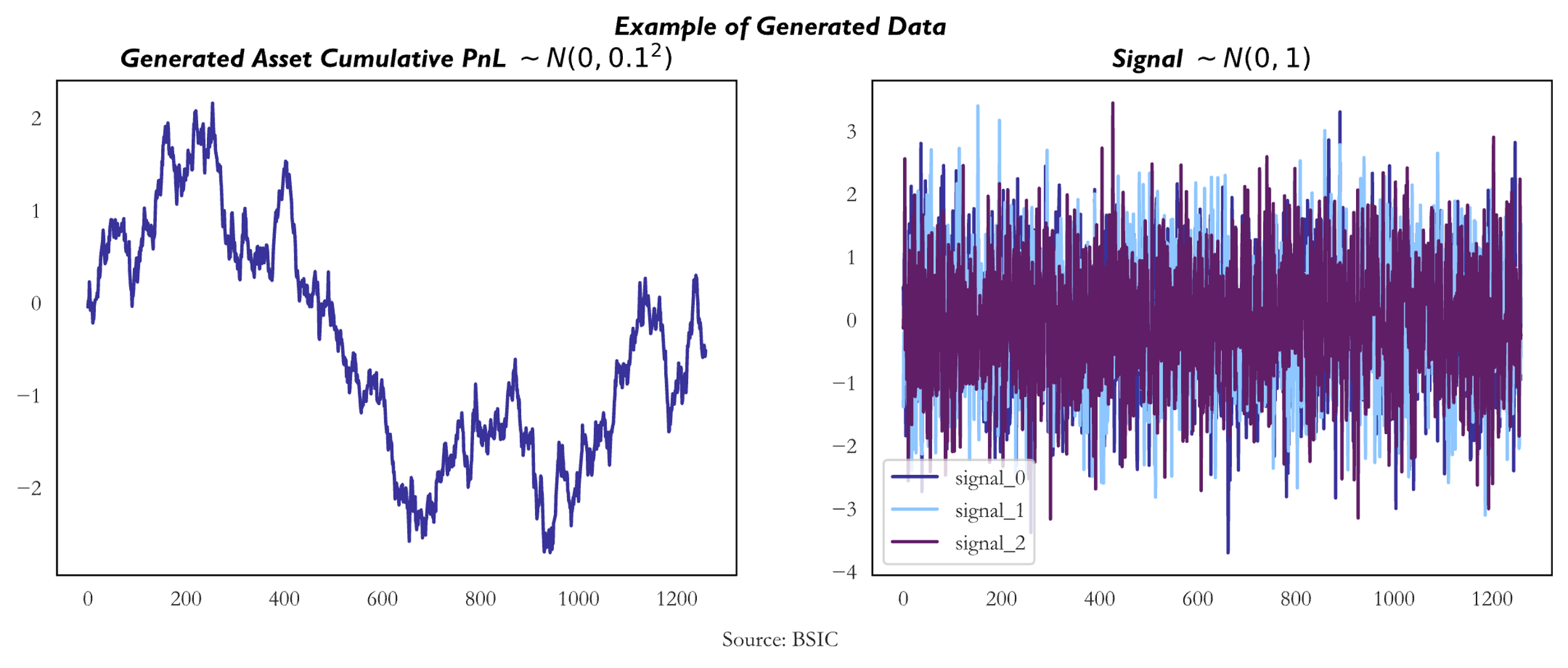
Generating Fictional Data

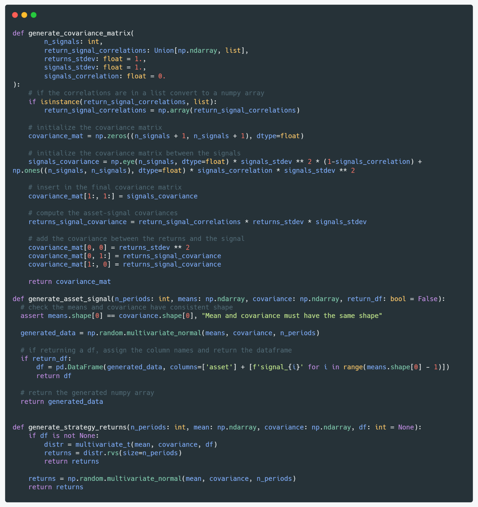
We need a robust way to compare the different methods we are going to propose over the series. We choose to simulate data, for the following reasons: (i) we do not have enough independent (and statistically significant) signals to test on, and creating them is outside the scope of the series, (ii) generating signals allows us to have a wider sample, and to know the true statistics that we are trying to estimate (SR, IC, IR…), (iii) generating signals allows us to impose different levels of correlation between the target and the alpha signals, and betweeen alpha signals themselves. We take the same approach as in Paleologo, 2024.

When generating alpha signals, we draw returns and signals from a multivariate normal distribution. We will tweak the vol of the asset, while keeping, without loss of generality, unit-variance for the signal (thus representing a z-score). We can set different correlations between the signals and the asset, and between the signals themselves. We can also generate strategy returns. In that case, we relax the assumption of normal returns and draw from a multivariate t-distribution, and we will tweak the correlation between the strategies, along with the correlations between them.

Conclusions

As we conclude this first episode in our series on backtesting, we’ve laid the groundwork by introducing key concepts to further develop our analysis. Understanding these fundamentals is crucial for building a robust backtesting pipeline. In the next episode, we will dive deeper into cross-validation techniques, exploring how to optimize the training and testing of your models to ensure more reliable results. Stay tuned as we discuss K-Fold and Walk-Forward validation methods, along with a novel approach using Rademacher Complexity, all of which are essential for refining your strategies and avoiding common mistakes in backtesting.

References

1. Grinold, Kahn, “Active Portfolio Management”, 1999
2. Paleologo, Giuseppe, “The Elements of Quantitative Investing”, 2024
3. Paleologo, Giuseppe, “Advanced Portfolio Management: A Quant’s Guide for Fundamental Investors”, 2021
4. Isichenko, Michael, “Quantitative Portfolio Management: The Art and Science of Statistical Arbitrage”, 2021
5. Chincarini, Kim, “Quantitative Equity Portfolio Management”, 2006
6. Pav, Steven, “The Sharpe Ratio: Statistics and Applications”, 2022
7. Andrew W. Lo “The Statistics of Sharpe Ratios”, 2003