Backtesting Series – Episode 2: Cross-Validation techniques

Download PDF

Introduction

As announced in our previous episode, the second article in our Backtesting series will discuss Cross Validation and introduce a new Backtesting strategy, first presented by Giuseppe Paleologo (2024). If you haven’t already, we recommend reading the first episode before proceeding with this article. Please note that the series will include the following parts:

• Part 1: Introduction
• Part 2: Cross-Validation techniques
• Part 3: Portfolio Construction & Portfolio Optimization, Factor Models
• Part 4: Backtest Analysis
• Part 5: Introducing TCs, assessing capacity, preparing for production

Cross-Validation

In Statistics Cross-Validation is a method to estimate a model generalization error. The goal is to avoid overfitting and understand how well the model will perform on unseen data. In a computational setting, it is possible to estimate the generalization error by splitting the data into two non-overlapping subsets: a training set and a holdout, or testing, set. To have a reasonably good estimate of the test (out-of-sample) error, the test data should be never used for training the model, large enough, and drawn from the underlying distribution without a bias.

In Cross-Validation the dataset is partitioned into several folds to validate a predictive model. It trains on the train set and then evaluates it on the remaining portion of the data, a test set. This whole process is repeated multiple times, but each time with a different fold as a test set, while the rest of the data is used as a training set. Doing so, Cross-Validation ensures the model is tested on different parts of the dataset, reducing the risk of overfitting and improving the estimate of performance on unseen data. Once all iterations are done, the results of different test subsets’ performances are averaged into an overall generalization performance of the model.

In time series analysis, Cross-Validation is more complex due to the temporal ordering of observations. Unlike standard Cross-Validation, where the data can be randomly shuffled, time series cross-validation must respect the inherent sequence of the data. Breaking this temporal order could lead to information leakage, where future values inadvertently influence the training of the model. We will present you two of the most recurrent Cross-Validation methodologies that are used in Backtesting.

K-fold

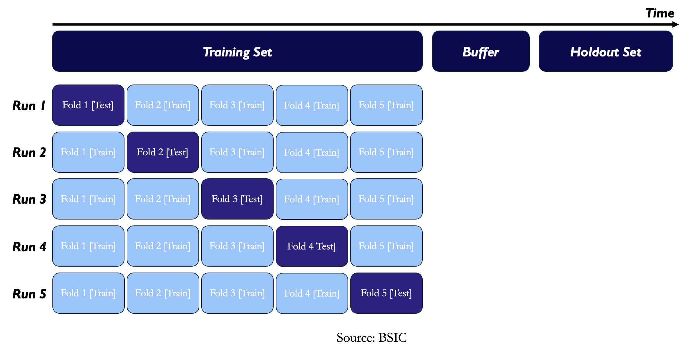
In K-fold cross-validation methodology the available data is split into a training dataset and a holdout or validation dataset. Keeping in mind that time series data can have time-dependent properties, a buffer period is used to separate the two sets with no overlap. The data is then divided into K equal-sized folds. To further reduce a potential dependence among those folds, even a small buffer could be set between them, too, as a remedy against look-ahead bias. Then we perform K estimation-evaluation exercises. The parameters are estimated on each of the possible combinations of K – 1 folds, and the performance of the model is evaluated of the remaining fold using the optimized parameter. Then estimate the cross-validation performance as the average of the single-run performances. Finally, performance is checked against the holdout sample.

Still, there are a lot of essential reasons why cross-validation is particularly problematic in the context of financial applications. First of all, financial data are not independent due to time dependencies inherent in asset returns. While the serial correlation of returns is usually weak and transient, the volatility dependence is much stronger and exhibits a long memory effect. Apart from those, certain predictors, take for example security momentum, add further complications to the cross-validation process. Momentum relies on historical returns, which creates a look-ahead bias when the temporal arrangement places the validation fold before the training fold. In this case, the historical returns used for the forecast of future performance are already part of the validation fold; hence, it allows the model to use future information in training.

Another main problem is that if you run Cross-Validation many times on different types of models, you’re bound to eventually get good results, even if they aren’t truly reliable. Indeed, if you test enough models or refine them over and overusing Cross-Validation, you’re likely to find a model that performs well just by chance. It may appear effective on Cross-Validation, but it might also just be overly tuned to the idiosyncrasies of the training data, not generalizing to truly unseen data. The purpose of a holdout dataset is to act as a final, unbiased check to prevent this kind of “fishing expedition” for favorable outcomes. However, when you’re dealing with millions of raw signals (features), it’s common to refine models repeatedly checking the holdout performance too many times. In this process, the performance on the holdout set can end up being treated like another parameter to optimize, rather than a one-time, independent test of the model’s true performance. The key idea here is that the holdout dataset should be used only once, after all model training and tuning are complete.

To better illustrate this, we present you a practical example on simulated data. We generated autocorrelated asset returns with , and . We then introduce random asset characteristics, also iid and drawn from . By construction these random features are not predictive of returns, and we will use them as signals. The Backtest consists in a 5-Fold Cross-Validation, to estimate the performance of the predictors. In each run, we select the best performing factor, based on in-sample IC, and then compute the IC on the test fold. Then we report the average cross-validated IC. We repeat the process on 1000 simulated data sets.

We experimented on two different scenarios:

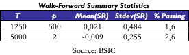
1. The first one is the “not many periods, more predictors” case: we set T = 1250 (five years of daily data) and p = 500.
2. The second one is the “many periods, not many predictors” case: we set T = 5000 (twenty years of daily data) and p = 2.

The histograms below show the two Sharpe Ratio distributions that we obtained from the simulation:

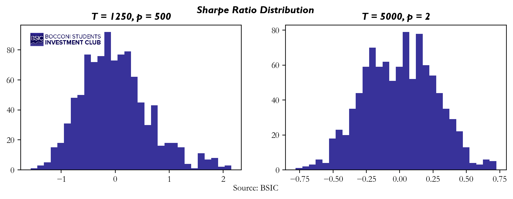
The frequency histograms indicate that the mean is close to zero for both scenarios, but there is a significantly higher standard deviation in the “not many periods, more predictors” case, with some Sharpe Ratios exceeding values of 2. What does this tell us? It suggests that if you over-optimize or backtest your strategy too many times on the same dataset and eventually achieve a high Sharpe Ratio, this does not necessarily mean you’ve discovered a market-beating strategy. Even features that are not predictive of returns can sometimes produce favorable results purely by chance. This means your high Sharpe Ratio might simply be the result of overfitting, and your strategy could lack robustness when applied to unseen data. Therefore, it’s crucial to be cautious and avoid reading too much into results that could be driven by randomness rather than genuine predictive power.

The variance suggests that the model, when exposed to many predictors but not enough historical periods, becomes more sensitive to randomness. While the mean remains close to zero, the wide spread of Sharpe Ratios indicates that even non-predictive features might seem valuable under certain conditions, further validating our concern.

Walk Forward

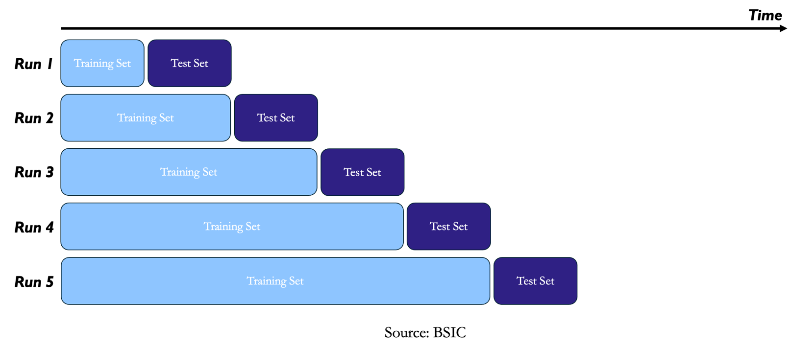
A remedy for look-ahead bias in K-fold Cross-Validation is Walk Forward Backtesting. Unlike standard cross-validation, where data can be randomly split into training and test sets, walk-forward cross-validation accounts for the temporal order of the data. In the scheme we start by training the model on an initial portion of the data, up to time t, testing it on the next block of time, and then expanding the training set to include the previous test set while moving forward in time. This process repeats until all data has been used for testing.

Walk-forward cross-validation eliminates two of the largest drawbacks compared with K-fold cross-validation: it addresses serial dependence and eliminates the possibility of look-ahead bias. Another appealing aspect is that it intrinsically walks the evolution of the dataset, naturally augments the dataset as new data becomes available, allowing the method to continuously adapt and update itself by incorporating the latest information. These advantages complement cross-validation, which is why simplified strategies or signals are often first evaluated using cross-validation and then tested “out of sample” with a walk-forward approach. This, however, is not very optimal, as it creates an opportunity cost due to the delay in putting the strategy into production.

Walk Forward has an additional drawback since it uses far less training data than K-fold and when the set of models and parameters is very large this limitation could be very severe. On the other side, when the model has been identified, and only a few parameters need to be optimized, this drawback becomes negligible.

Finally, walk-forward backtesting has a high overfitting risk concerning the trading strategy, in comparison with other methods of conducting tests, such as the K-fold Cross-Validation. This is because the model may have learned patterns that are specific to the historical dataset rather than general trends. Walk-forward testing splits data into multiple training and testing periods, so there’s always a risk of over-optimizing the strategy to each small segment of historical data. Since this method does not use all the data at once and adapts after every walk-forward iteration, it might encourage the selection of complex strategies that work very well on a particular segment but perform poorly in real-world conditions. Therefore, over-complexity in the model increases the possibility of overfitting to the historical data at the cost of the performance in the future.

To better explain this, we repropose you the same practical example used in K-fold Cross-Validation, this time using Walk Forward Backtesting. Here are the results we got:

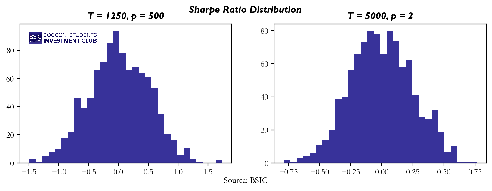
The results presented here are quite consistent with what we observed in the K-Fold Simulation. In both cases, the histograms demonstrate a mean that hovers around zero. However, the scenario characterized by “not many periods, many predictors” shows again a noticeably higher variance compared to the other scenario. This finding aligns well with our initial assumptions regarding the risks associated with over-refining models based on a limited holdout dataset. The increased variance in this scenario underscores the danger of repeatedly tuning models on the same data leading to overfitting and generating unstable results.

Considerations on Cross Validation methodologies

Ideally you would like your Backtesting protocol to have the following properties:

1. Non-anticipative and immune from look-ahead bias;
2. Takes into account serial dependencies;
3. Uses all the data;
4. Allows for multiple testing of a very large number of signals;
5. Provides a rigorous decision rule.

As previously introduced, Walk Forward Backtesting meets the first two requirements while K-Fold cross validation meets the third, although none of the two, neither if combined, satisfy all the properties of an ideal backtesting protocol. We will now present you a new Backtesting Methodology that tries to meet all of them at once.

Rademacher Anti-Serum

As extensively mentioned in the previous two sections, both K-fold and Walk-forward techniques have important drawbacks that can hardly be overlooked when back testing a strategy. This, paired with the fact that some performance measures like Sharpe Ratio are inherently biased (as explained in part 1), may cause our estimates for performance of certain strategies or signals to be inherently biased. To account for this, we report the use of a novel method developed by Giuseppe Paleologo, called Rademacher Anti-Serum. The method effectively allows practitioners to have a mathematically robust lower bound on the real performance of their strategy, starting from its sample estimate. For ease of comprehension to the reader, we will report the main components of the framework, as well as the most relevant results and their underlying intuition. For a more rigorous argument on why such results hold, we encourage the readers to go through the passage on the latest book from Paleologo himself [2].

As mentioned in the introduction to the section, we are interested in analysing the performance of strategies of alpha signals. For this purpose, we can use either Empirical Sharpe Ratios or Information Coefficients. Below the formulas for them, in matrix form:

Where is our weights for strategy at time and similarly for .

In general, we can consider a matrix of size where each element represents a certain strategy/signal at a specific time.

Let and respectively represent the rows and columns of our matrix. Note that we assume the rows to be i.i.d. and to be drawing from a common probability distribution , meaning that each row is not serially correlated through time. Assume that , where is the vector of true performances. Normally, the true parameter is unknown, and hence we need to recur to its sample estimation:

To have a better understanding of the true from our empirical one, we introduce the concept of Rademacher Complexity:

Let This will be referred to as a Rademacher vector and has dimension . From this, Rademacher Complexity is so defined:

Such a metric has some very interesting interpretations.

• We can firstly intend it as “covariance to random noise”. Since is by all means like moving according or opposite to our strategy n, having a high Rademacher Complexity is like to say that, given our portfolio of strategies/signals, we can always find a good strategy that covariates with pure random noise. It is clear that, if effectively we always have a “good strategy” whatever randomness we encounter in reality, we are probably grossly overfitting in our back testing. As a matter of fact, one can easily show that the higher the number of signals and the lower the correlation between them, the higher will Rademacher Complexity be. This is, again, quite intuitive (and will be shown in the later section with our simulation). Indeed, the more orthogonal are the strategies between each other, the higher the likelihood that at least one correlates decently to pure random noise.
• The formula itself can also be intended as a 2-way cross-validation. Indeed, as T increases, we can easily assume a 50-50 division of negative and positive values (let and respectively represent these two subsets). One can then decompose the inner part of as:

Since we are taking the of this measure, it is quite clear that actually we are taking the one strategy with the highest discrepancy, meaning it performs very well in some subset and fairly poorly in others. If this is high for any random subset (since we are taking ) the performance is not consistent, and hence it has unreliable performance (and thus higher complexity).

• Assuming that we use as performance measure Sharpes (i.e., standardized returns), we can say that is strongly concentrated around and a similar argument can be made for the norm of . This means that we can approximate our empirical Rademacher as follows:

which has some interesting interpretation. Indeed, is nothing more than a random path or direction in and for a set of performance vectors we observe the maximum collinearity of this random path to our vector, which basically represents how much our set of strategies spans . Clearly, this is to say that the more orthogonal our set of strategies, the better they will span .

More importantly, however, we can apply the use of this metric, when trying to obtain a more realistic lower bound on our initial true for each strategy/signal, starting from the sample estimate and removing a “haircut”, obtaining the following relationship (refer to [2] for the proofs of this):

• In the case of signals and thus information coefficients:

Where represents our probabilistic guarantee on the true parameter (e.g., 99% certainty lower bound)

• In the case of Sharpe Ratios:

The first term, in both formulas, is what can be defined as a “data snooping term”. Indeed, as we extensively covered, being dependent on it grows both in number of strategies and proportionally to the orthogonality among the strategies themselves. Computationally, an upper bound for estimated .

The second term, instead, is effectively an “estimation error”. Very importantly, this error does not depend on the number of strategies N in the case of bounded distributions (like I.C., which is clearly bounded since it represents a correlation), while is for sub-Gaussian distributions like in the case of Sharpe Ratio.

In the following section, we will set up a simulation for a portfolio of signals and prove empirically that these relationships hold. This will serve as a proof of concept of how this procedure might be used in a more practical setting.

Simulations

It follows from the definition of Rademacher Complexity that this value should vary depending on the correlation between signals (or returns), as well as on the number of strategies. Why does this happen? First, as the number of strategies increases, the likelihood that at least one of them will fit the random noise also increases. Therefore, in general, Rademacher Complexity tends to increase with N. On the other hand, the Rademacher Complexity shall decrease in as if signals are highly correlated, it becomes more difficult to find a strategy that stands out from the others and outperform in terms of fitting the random noise. To prove that we ran a simulation on different values of N and to see how the Rademacher Complexity’s value changes.

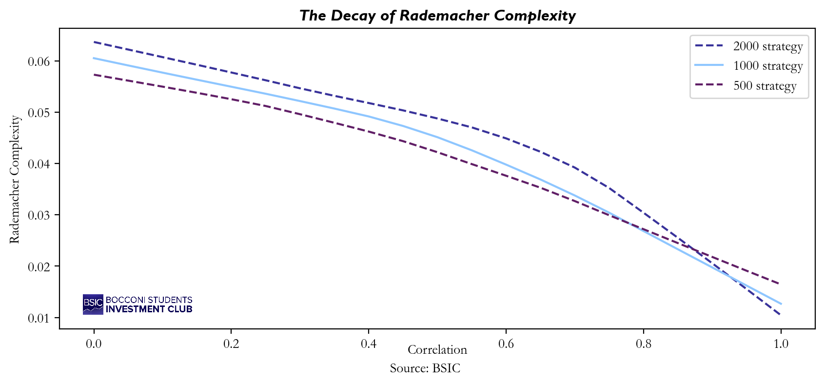
As expected, the higher curve is the one of 2000 strategy, proving that Rademacher Complexity is actually increasing in N. Instead, from all three curves we can deduce that not only the Rademacher Complexity is decreasing in but also that as then .

Then, to evaluate the performance of Paleologo’s approach, we conducted tests using simulated data. Specifically, we generated excess returns and alpha signals from a multivariate normal distribution while maintaining unit variance for the signals. Following this, we constructed our matrix by computing information coefficient for each of the N strategies using a walk-forward procedure. This setup allowed us to simulate different scenarios by varying the correlation between signals themselves and and the correlation between the signals and the asset’s excess returns. Additionally, we examined various combinations of the number of strategies and the number of time periods to explore a broader range of conditions.

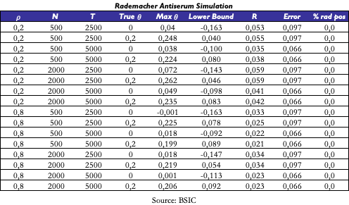
For each simulation scenario, we computed several key metrics. First, we recorded the maximum empirical value of , the Rademacher Complexity (R), the estimated error and the lower bound on (calculated on a 99.9% confidence interval). We also report the “Rademacher positive” strategies, i.e., the strategies that exceed the data snooping term alone, in formula those strategy for who’s the following relationship holds:

In summary our aim is not only to assess how Rademacher Antiserum estimates the predictive power of the signals but also explore how different levels of correlation and strategy diversity impact model performance and reliance.

Here there are e few considerations on the results we got:

1. The max empirical is predictably increasing in N, as a larger number of strategies increases the likelihood that at least one will align well with the data. Conversely it is decreasing in as higher correlations among signals reduce the chance that any single signal will outperform the average, and finally it is decreasing in T, by the Central Limit Theorem, since larger sample sizes tend to smooth out fluctuations.
2. Everything else equal, the Rademacher Complexity is decreasing in implying that with higher correlation is less likely to find a strategy able to fit the noise, i.e. the Rademacher Vector. Instead, it is increasing in N and decreasing in T.
3. The discrepancy between the and the Lower Bound can largely be attributed to estimation error, which, within a 99.9% confidence interval, is quite substantial and conservative. However, even when we focus solely on the data snooping correction term, it is important to highlight that the percentage of Rademacher Positive strategies remains consistently at 0 across all parameter configurations tested.

Conclusions

In this article, we explored two of the most widely used cross-validation techniques, K-fold and Walk Forward, and discussed their respective strengths and limitations when applied to financial time series data. Both methods are valued, but neither fully addresses the challenges of financial modeling with the risks of look-ahead bias, serial dependence, and the intrinsic limitations of Backtesting in small or noisy datasets.

On the other hand, Rademacher Anti-Serum method presents an innovative approach, providing a robust lower bound for strategy performance while accounting for overfitting. As we have shown through simulations, the Rademacher Anti-Serum proves particularly useful in handling large sets of strategies and signals. It counters the risks posed by K-fold’s overuse of small training sets and walk-forward’s tendency toward model overfitting across different time segments. Moreover, this methodology allows to use all the data available and provide a rigorous decision rule.

In our next episode, we will delve into Factor Models, a critical framework in portfolio construction and optimization. Factor Models allow for a deeper understanding of the risk and return drivers behind asset performance. Stay tuned as we will delve deeper into this crucial topic of quantitative investing.

References

1. Paleologo, Giuseppe, “The Elements of Quantitative Investing”, 2024
2. Michael, Isichenko, “Quantitative Portfolio Management”, 2021
3. Grinold, Kahn, “Active Portfolio Management”, 1999