Introduction
Financial instruments related to carbon emissions have been described in the past two years as a “one-way” bet for hedge funds and other financial players, who think the value of these contracts will rise in the future. The rationale behind these products is that negative externalities like pollution, not reflected in market prices, should be internalized. There are two main approaches to carbon-pricing systems: Carbon Tax Regimes, in which a price on carbon is set directly by defining a tax rate on greenhouse gas (GHG) emissions, and Market-based Systems. In Market-based Systems, which we are going to discuss in this article, the supply and demand of specific carbon emissions permits largely determine the cost of polluting.
Market-based Systems are divided into Cap-and-Trade Systems and Baseline-and-Credit Systems. Under the former, regulators set a cap on the total amount of GHG emissions companies can produce each year. If a company pollutes more than the cap level, then it needs to buy carbon permits, also known as carbon allowances. The regulators distribute these allowances in part freely and in part monetize them via auctions. Both physical emitters and financial players can exchange these allowances on the derivatives markets. The EU ETS (Emissions Trading System) is an example of cap-and-trade systems. Under baseline-and-credit systems, there is no fixed limit on emissions, but polluters that reduce their emissions more than they otherwise are obliged to can earn carbon credits. The credits can be sold to other companies who need them in order to comply with regulations they are subject to. For instance, Stellantis bought about €2 billion of European and U.S. carbon credits from Tesla between 2019 and 2021.

Source: Bloomberg, Bocconi Students Investment Club
The recent surge in price of these contracts, specifically of the EUA futures, has been remarkable. From a pandemic low of EUR 23.03 per metric ton, they have risen above EUR 60/mt. This rise has led Bloomberg to describe the situation as an “expensive mess”, given the current energy supply crunch that Europe is facing, and limited production of renewable energy caused by slower wind in the North Sea. Before we investigate price determinants more in depth, let us provide a brief yet useful historical background to the contracts at hand.
The EU Emissions Trading System
Set up in 2005, the EU ETS market is the world’s first international emissions trading system, where EU Allowances (EUA) are traded. The EU ETS accounts for some 75% of global carbon emissions market turnover and 85% of its market value. It is operational across all 27 member states and European Economic Area countries Norway, Iceland, and Liechtenstein. In January 2020, the EU ETS was linked to the Swiss ETS. Following the UK’s departure from the EU, a UK ETS became operational in May 2021 and may be linked to the EU ETS.
The EU ETS market went through many phases. Phase 1 (2005 – 2007) was characterized by:
• only CO2 emissions from power generators and energy-intensive industries were covered in this period
• almost all allowances were given to businesses for free
• the penalty for non-compliance was $40 per ton
In the absence of reliable emissions data, phase 1 caps were set on the basis of estimates. As a result, the total amount of allowances issued exceeded emissions and, with supply significantly exceeding demand, in 2007 the price of allowances fell to zero (phase 1 allowances could not be banked for use in phase 2).
Key features of Phase 2 (2008 – 2012) were:
• lower cap on allowances (some 6.5% lower compared to 2005)
• the proportion of free allocation fell slightly to around 90%
• the penalty for non-compliance was increased to €100 per ton
• businesses were allowed to buy international credits
Because verified annual emissions data from the pilot phase was now available, the cap on allowances was reduced in phase 2, based on actual emissions. However, the 2008 economic crisis led to emissions reductions that were greater than expected. This led to a large surplus of allowances and credits, which weighed heavily on the carbon price throughout phase 2.
The reform of the ETS framework for Phase 3 (2013 – 2020) changed the system considerably compared to Phase 1 and Phase 2. The main changes included:
• an EU cap system on emissions in place of the previous systems of national caps
• auctioning as the default method for allocating allowances
• a linear reduction factor (LRF) of 1.74% per year to the EU emissions cap, meaning that each year supply of allowances was reduced by around 40 metric tons (Mt)
• introduction of Market Stability Reserve intended to address the oversupply of allowances
Now there is Phase 4, going from 2021 to 2030, whose aim is to reduce GHG emissions by 50-55 percent from 1990 levels, up from the previous target of 40 percent. Regulators will be bolder, announcing an increase in the LRF to 2.2% per year, the inclusion of shipping in the EU ETS and the CBAM, a custom levy on the carbon content of imported goods, will be phased in, while free allocations to selected industries will be phased out.
Analytics and Price Determinants
As we mentioned earlier, a huge surge in prices has unfolded recently in emissions trading markets. Displayed below is a chart with the futures curve on EUA contracts 1 week ago, 1, 3 and 6 months ago, and 1 year ago. A clear pattern of upward pressure is evident, indicating that the expectations of market participants concerning the future price of emission allowances are more “bullish” than ever.

Source: Bloomberg, Bocconi Students Investment Club
If we look at how the price has evolved in relationship with other energy commodities, we get the following picture:

Source: Bloomberg, Bocconi Students Investment Club
Leaving aside for a moment the trend divergence of EUA futures quotes with the TTF Natural Gas and the Coal prices in the last 3 months, it appears that the above displayed time series might prove useful in a study of the price determinants of EUA. Thus, we now present a more formal analysis of the drivers of these contracts.
To understand the price determinants of EUA futures, we apply some econometric methodologies that focus on the association of the time series of EUA futures quotes with other commodity price time series. We use price data from the past 6 years for Brent Crude, TTF Natural Gas, Henry Hub Natural Gas, Coal, Electricity (all front-month futures), the Stoxx 50 index, GSCI, and the MSCI World.
We start with correlation. To do so, we must firstly ascertain that the time series be stationary, namely that they have time-invariant first and second moments, because correlation is a linear measure of association, and the presence of a trend would hinder that analysis. To do so, we apply the Augmented Dickey-Fuller test in Python, which tests the null hypothesis that there is a unit root (i.e., that the time series exhibit order of integration equal to 1). As we could expect, all the time series exhibit a unit root and thus are nonstationary. We address this issue through differencing. Displayed below is the correlation matrix we obtain:
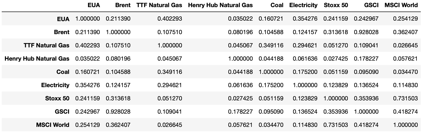
Source: Bocconi Students Investment Club
This simple analysis yields some interesting insights. We focus on the first row (or, equivalently, the first column) as the others don’t pertain to EUA contracts’ correlation with other assets. Firstly, we notice that EUA futures are most strongly correlated with the price of Dutch TTF, and least correlated with that of Henry Hub. This is far from surprising, as TTF represents the benchmark for European natural gas, whereas Henry Hub is a distribution hub in Erath, Louisiana (US). The second-strongest correlation, quite unexpectedly, is with electricity prices, with a coefficient equal to 35.43%. A potential explanation for this relationship will be discussed when we present the Granger causality test. Then, positive and nonnegligible correlations are found with the Stoxx 50, MSCI World and GSCI. A potential econometrically-inspired motivation for this is that those three indices might be serving as instrumental variables for the economy. In other words, those correlations might be due to the betas that those major equity and commodity indices exhibit to the strength of business and firms. Then, it makes sense that they would be positively correlated with emission prices, since the greater economic activity causes emissions to go up. Finally, Brent crude is correlated with EUA futures with a coefficient of 21.14%, while the coefficient for coal is just 16.07%. The latter number might be understood if we conjecture that higher coal prices might reflect higher demand for coal, and being it the strongest polluter, emission allowances would have to go up as well.
However, correlation is not causation. Therefore, we need to use more advanced metrics to understand the type of association between EUA futures quotes and other commodities. We can get one step closer to establishing causation by testing for cointegration. Cointegration is the property of time series of order of integration d for which there exists a linear combination whose order of integration is lower than d. The intuition is that, if two series that exhibit a unit root are cointegrated, the spread (difference between the values of the two series at each time step) is stationary, i.e., it has constant mean and variance.
Since the Augmented Dickey-Fuller test described above showed that all the time series are of the same order of integration (1), we can test for cointegration. The results from the Engle-Granger two-step cointegration test indicate that none of the price series of the above-listed commodities is cointegrated with the EUA futures quotes series. This has an important implication, namely that pairs trading between EUA futures and any of the other commodities would be very difficult to implement.
Arguably, the last step we can take in testing for causality is the Granger test, which we can apply since we have differenced the data, obtaining stationary time series. The Granger causality test assumes that causality can be tested for by determining whether a time series can predict future values of another time series. In other words, a time-varying random variable X is said to Granger-cause another time-varying random variable Y if past values of Y and X are better at predicting future values of Y than past values of Y alone. The results of the test are displayed below.
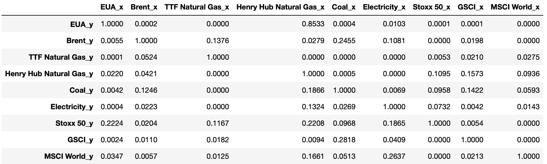
Source: Bocconi Students Investment Club
The table above displays p-values. The null hypothesis of the Granger test is that one time series doesn’t Granger-cause the other, thus p-values above (1 – confidence level) indicate that there is insufficient evidence to reject the null hypothesis, and Granger causality cannot be asserted. Consider for instance the p-value for the test where the Henry Hub price is used as a predictor for EUA quotes. It is equal to 0.8533, which implies that the null hypothesis cannot be rejected with any sensible confidence level (generally chosen to be 95% or even 99%).
The results indicate that Brent Crude, TTF Natural Gas, Coal, Electricity, the Stoxx 50 index, the GSCI and the MSCI World index all Granger-cause the price of EUA futures contracts. From this, we can infer that when all the time series except for Henry Hub prices are used to predict/explain EUA futures prices, for instance in a vector autoregressive (VAR) model, we get better results than if we used a simple autoregressive model based on EUA futures quotes alone. Furthermore, it appears that Granger causality for electricity and EUA quotes is stronger when EUA quotes are used as a predictor of electricity prices. This might suggest that the very strong correlation discussed earlier between the two time series can be motivated by a dynamic whereby when emissions become more expensive, producers tend to switch to electricity, a less polluting energy source, insomuch as they can, thus driving up the electricity price.
As a final note, we remark that the presence of Granger causality is entirely compatible with the absence of cointegration (as is the case with our data), while the opposite is not true, as the presence of cointegration requires Granger causality to hold in at least one direction.
Conclusions
It should be noted that the price for EUA is largely determined by supply and demand in the short term, with utilities and industrial operators subjected to EU ETS compliance being the most active operators in the markets instead of hedge funds or investment firms, often cited by media outlets. However, in the long run, the regulator could be the driving force of this market. According to the Paris Climate Agreement, the price to be set for carbon in order to reduce GHG emissions below the desired level is higher than $100. A high price for carbon should incentivize polluters to switch to clean energy production systems and reduce their emissions. Therefore, financial players are piling into carbon credit markets because they believe the regulator will end up aligning the market price to its long-term goals by setting a lower cap and controlling supply of allowances.


0 Comments