Introduction
The perfect storm of harsh macroeconomic conditions and geopolitical uncertainty has taken its toll on the markets. 2022 saw widespread selloffs across all asset classes and is considered to be one of the worst years on record for investors. Although the equity markets have fared worse through previous financial crises (2000, 2008, and 2020), what makes this year’s market performance so destructive is that all asset classes are down. Systematic risk has been the main cause of asset depreciation and investors are struggling to generate alpha in portfolios. In this article, we discuss the reasons behind why historically negatively correlated assets are now trading inversely and how investors can succeed in the current market conditions through trades isolating correlation.
Correlation Trends Across Asset Classes
The main driver of recent correlation shocks to equities and fixed income is inflation – and central bank activity as a result of it. With the most recent CPI print coming in at +7.7% for October, monetary policy continues to dictate valuations and the trading environment.
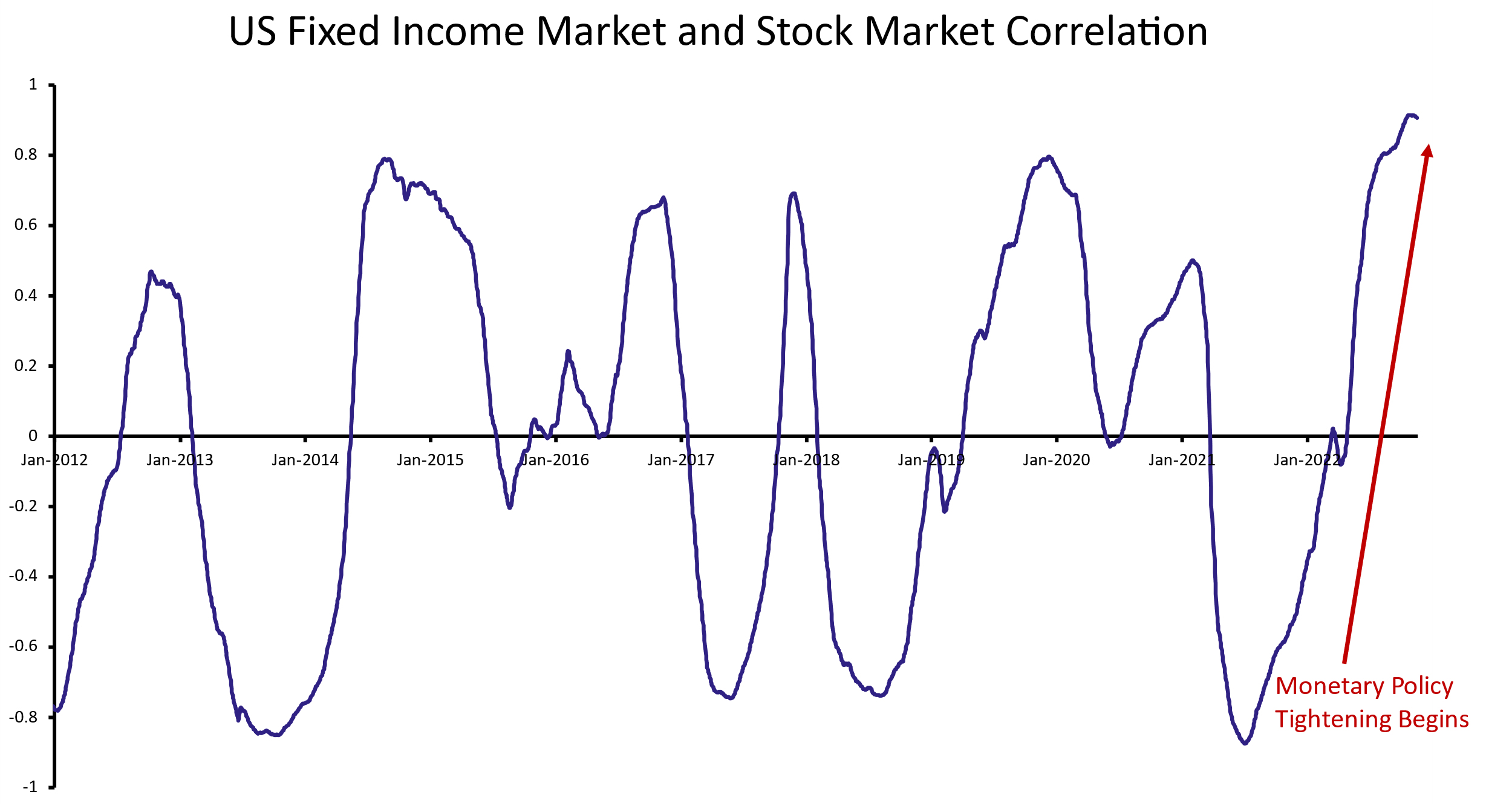
Historically, equities and fixed income have seen low positive correlation, and even commonly negative correlation. However, the correlation between these two asset classes has steadily increased in recent years and is now at a decade high. Year-to-date, the S&P 500 is down -17.33%. One would expect this to spark a flight-to-safety towards fixed income, however, the 10-year treasury is also down -16.54% (as proxied through the S&P U.S. Treasury Bond Current 10-Year Index). In the chart below, we calculate the one-year rolling correlation between the S&P 500 and Vanguard’s Total Bond Market Index Fund ETF to compare how stocks have performed in comparison to the government and corporate bond market.
Source: Yahoo Finance, Bocconi Students Investment Club
Now taking a broader view into the FX markets, traditionally, the dollar and the US stock market have been positively correlated. Although there are a many factors driving the dollar’s performance, 40% of the time, the S&P 500 and the US dollar will rise together. The main explanation for this occurrence is foreign investment. In order for international investors to purchase US equities, they must first purchase US dollars. However, in today’s inflation-dominated markets, increasing interest rates have pummeled equities while pulling the dollar higher and therefore breaking the correlation. Recently, the dollar tumbled thanks to the first hints of slowing US CPI which has broken its strengthening of almost 25% since 2021. Unsurprisingly, equities rallied with the S&P 500 up 5.5%, its strongest one-day gain since April 2020.
The Key Driver of Correlation
Higher inflation is currently the key explanation as to why equities and fixed income are positively correlated. Central banks are responding to inflation by tightening monetary policy. As both asset classes have exposure to short-term interest rates, they are negatively affected as a result. Fixed income directly takes a hit from rising interest rates as bond prices and yields are inversely related. Additionally, the higher interest rates also eat away equity valuations through an increase in the risk-free rate, combined with slowing corporate earnings through a tightening economy. Clearly, this is a painful combination for investors as diversification no longer plays the role that it used to in lowering risk in portfolios. As a rule of thumb, correlation tends to surge in times of market crises, where macroeconomic risks govern the markets across all asset classes.
Correlation and Portfolios
As introduced in the previous section, the benefits of diversification are no longer as evident due to correlations breaking away from historical trends. The 60/40 portfolio, also known as a balanced portfolio, is made up of 60% equities and 40% bonds. This portfolio mix was a pillar of portfolio construction in the 1980s and 1990s because it provided attractive risk-adjusted returns. What made the portfolio successful was that equities would be the main driver of returns and bonds would offset losses during times of market crises (e.g. the dot-com bubble burst), thanks to its negative correlation. However, it required a very specific macroenvironment to be successful: low inflation, falling real yields, and an accommodative Fed. The last time the markets saw high inflation was in 1981 where year-on-year CPI came in at 10.3%. Since then, inflation has been under control and has averaged at a year-on-year increase of 2.7% from 1982-2021. With low inflation came low yields and low correlation between equities and fixed income, supporting the benefits of diversification in 60/40 portfolios. Next, as real yields (or inflation-adjusted yields) had consistently fallen between the 1980s and 2021, equity and fixed income valuations have grown as yields and prices are inversely related. Finally, an accommodative Fed sparked investor confidence in the markets and in future economic growth, which contributed to a risk-on environment.
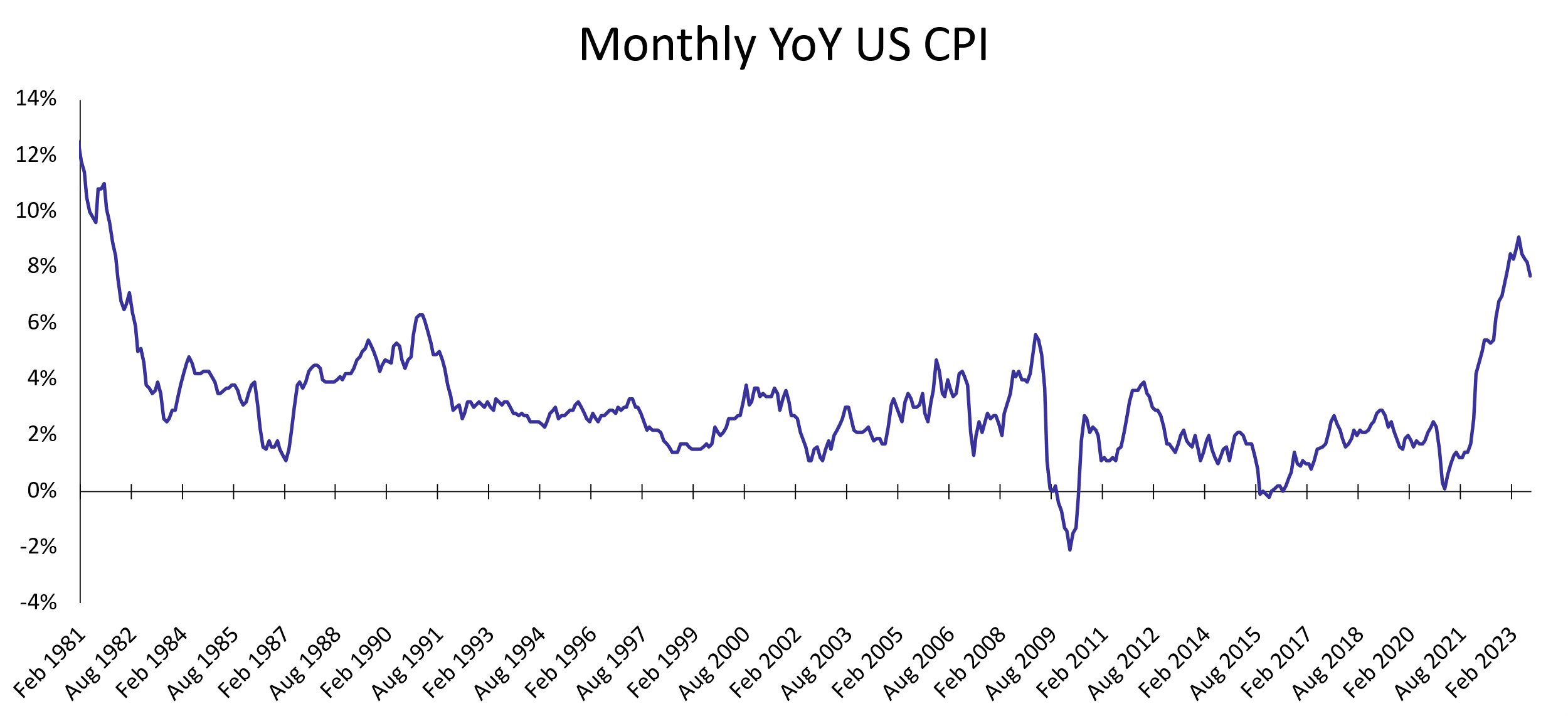
Source: US Bureau of Labor Statistics, Bocconi Students Investment Club
In a market regime change like the one that we are seeing today, a 60/40 portfolio faces strong headwinds. Investors are looking for new ways to diversify portfolio risks and are shifting away from this asset allocation mix. The Yale University Endowment Fund is a prime example as only 26% of its portfolio is invested in public equities, and 8% in fixed income. However, back in 1989, almost 75% of the endowment was in US stocks, bonds, and cash. “The Yale Model” is the fund’s investment strategy as developed by the former endowment director, Dean Takahashi. The model focuses on broad diversification and prefers alternative investments such as private equity, venture capital, hedge funds and real estate to traditional assets like stocks and bonds. Yale abandoned the 60/40 portfolio ages ago and that led to its 40.2% investment return in 2021. 2022 poses an interesting investment environment for the fund as the majority of its portfolio is not exposed to market risk.

Source: Yale Investments Office, Bocconi Students Investment Club
Trading Correlation
Correlation trading can take on many different forms depending on the goal of the investor, as well as the liquidity needed. We explore the most common trades below.
Correlation Swaps
A correlation swap is an exotic derivative that monitors the correlation between two (or more) assets at a specified future date. It is particularly complicated as the parties involved must predict how the prices of the two assets will change in relation to one another. The payoff of a correlation swap at maturity is the difference between realized correlation and the strike, where realized correlation is made up of historical correlation and future realized correlation. Ultimately, correlation swaps allow investors to take views on future realized correlation against implied correlation. The buyer of a correlation swap receives realized correlation and pays the strike at maturity; they benefit from correlation increasing.
Correlation swaps were first traded in 2002 as a solution for investment banks to hedge their short correlation exposure. For example, an investment bank has a position in stock A and stock B. These positions result in a net gain of $100 per 0.1-point increase in correlation (and a net loss of $100 per 0.1-point decrease). To remove this correlation risk, the bank could enter a correlation swap in the offsetting direction, where the bank loses $100 per 0.1-point increase in correlation. The resulting aggregate position has no correlation exposure.
There are no arbitrage-free standardized pricing models for correlation swaps currently available. However, a correlation swap’s cash flows are more similar to those of futures than vanilla swaps since its payoff can be calculated as the difference of the realized correlation and the strike. Depending on whether the correlation swap is an equal weight correlation swap or a market value correlation swap, the payout can be calculated as follows:

where
Notional = notional amount paid, or received, per correlation point
 = strike of correlation swap
For equal weight correlation swaps:

For market value weight correlation swaps:
![[\rho = \frac{\sum_{i=1, j>i}^{n}w_i w_j \rho_{i_j}}{\sum_{i=1,\ j>i}^{n}w_i w_j}]](https://bsic.it/wp-content/ql-cache/quicklatex.com-09eec024ef63fe9e8cfb14c7e5796be1_l3.png "Rendered by QuickLaTeX.com")
where
n= number of strikes
Since then, correlation swaps have been used for both hedging and speculative purposes as they are considered one of the most direct strategies for correlation exposure. However, there is less investor demand for correlation swaps, resulting in a highly illiquid market. This leads to multiple issues, such as difficulty closing positions and marking positions to market.
Dispersion Trading
Dispersion trading consists of being short index options/volatility and long options/volatility of the components of the index (and vice versa). All trades are dynamically delta-hedged over the entire horizon of the trade. Dispersion trading allows investors to profit from price differences between index options and options on the individual stocks when there are shifts in correlation between them. It is the most common method of trading implied volatility as the liquidity of vanilla options – especially those of indices and large cap stocks – is high. However, in contrast to correlation swaps that are pure correlation, a dispersion trade is dependent on volatility and is short volga.
The P&L of a dispersion trade is as follows:

Although dispersion trades are always short index volatility and long single stock volatility, there are three main strategies for determining the ratio between the two legs: theta weighted, vega weighted, and gamma weighted. Theta-weighted dispersions are the best weighing for achieving nearly pure correlation exposure, as its P&L is largely driven by the difference between implied and realized correlation. As seen in the P&L formula above, the payout equals the difference multiplied by the weighted average variance. With constant volatility and zero volga, the payout of the dispersion trade equals the payout of the correlation swap.
Basket Options
Basket options are financial derivatives where the underlying is a basket (portfolio) of assets. Similar to single-stock options, a basket option provides the holder the right, but not the obligation, to buy or sell the basket on or before the maturity date. The strike price is calculated by taking a weighted average of the prices of its components. Due to basket options trading over the counter, advantages it provides are its bespoke form to investors, and lower transaction fees since the entire basket is one trade. Basket options that have the same members and respective weightings as an index are nearly identical to an option on the index. However, the members and their weightings in a basket cannot change. They are the most liquid correlation product.


where
K = the strike
The most popular basket option is on two equal weighted indices. The payout of basket options is based on covariance which is the correlation multiplied by the volatility of the two underlying assets.
Covariance Swaps
Covariance swaps consist of forward contracts on two underlying assets and pay the difference of the realized covariance of the two assets over a fixed strike. The buyer of the covariance swap is long covariance, and therefore the volatility and correlation between the assets. The payout is correlation multiplied by the volatility of the two assets. One disadvantage to this trade is that it is difficult to hedge because there is no general static replication formula and limited liquidity.
The covariance swap payoff is as following:
![[Covariance(A,B)-K_{covariance}]\times Notional](https://bsic.it/wp-content/ql-cache/quicklatex.com-46a6692350090715bcf56d9d6c1d91da_l3.png "Rendered by QuickLaTeX.com")
Worst of/Best of Options
Worst of/best of options are bundles of call or put options with the same expiration dates but on different assets. On the expiry date, the option of the worst/best performing asset will be exercised if it is in-the-money. Liquidity in best-of options is very low although there are some buyers for best of call options. Additionally, worst-of puts are more expensive than any puts on the underlying. Worst-of/best-of options are the most common products involving correlation as they are popular light exotics.
Outperformance Options
Outperformance options returns are based on the difference in returns of the two underlying assets. They are cheaper than options on both individual assets and are short correlation.
Same Asset Correlation Swaps
Correlation swaps can be structured to include cross asset correlation exposure through a mix of commodities, equities, and foreign exchange. However, they are incredibly illiquid and carry large premia as investment banks would have difficulty hedging their positions. Due to these reasons, correlation swaps are most commonly traded within the same asset class.
Equity correlation swaps are traded using large indices and/or their components, the underlying equities can be, however, from different countries with different currencies such as Nikkei and S&P500.
The most liquid application of a correlation swap is in foreign exchange. FX markets allow structurers to easily find the correlation of the currency pairs due to the amount of reported data. Additionally, as currencies are expressed in relation to another, correlation is already implicit in a trader’s view. This results in lower premia being demanded, and the ability to exit a position before the expiry date.
Trade Idea: EURUSD & NOKUSD Short Correlation Swap
Thesis
We are pitching a correlation trade between EURUSD and NOKUSD through a short correlation swap with a one-year expiry. We believe that over the next year, there will be a decrease in correlation of the two currency pairs due to diverging monetary policy between Norway and Europe. The ECB is likely to turn dovish before the Norges Bank does, as a result of political pressures from unstable members of the Eurozone. This combined with the other factors listed above should result in a significant break in the correlation of the two currency pairs.
The trailing twelve-month correlation (as of October 19th, 2022) of the two currency pairs is 0.927, and year to date it is realizing at 0.932.
Catalysts
Norwegian Gas Exports Drive NOK Strength. Following the halt of gas exports from Russia, Norway has become one of Europe’s largest suppliers. Norwegian gas exports will continue to gain market share of European gas imports, as the US and Qatar have limited supply due to a lack of export infrastructure. The European Union will need to replenish its gas reserves over next year and is likely to increase imports from Norway, providing significant upside to the NOK.
Increased Geopolitical Uncertainty in the Euro-Zone. Consensus estimates for how long the Russia-Ukraine war will continue have increased over the duration of the war. This creates prolonged geopolitical uncertainty to the European Union, and especially to countries neighboring Ukraine and Russia, which will weaken the Euro.
Weakening European Economies. October saw hot inflation of +10.6% year-over-year in Europe and is expected to persist. Whereas in Norway, it was relatively slower at a rate of +7.5%. The Norges Bank can be expected to act more hawkishly compared to the ECB due to Norway having lower debt-to-GDP ratios (43.2% compared 97.7%). The ECB is unique as some countries in the Eurozone have elevated debt ratios and cannot sustain higher interest rates (e.g. Italy’s debt-to-GDP ratio of 154.2%). Additionally considering that the ECB President, Christine Lagarde, has said that a deposit rate above 2% is “restrictive”, which is a negative real interest rate of more than 8%, the ECB is unlikely to hike rates higher than other central banks such as the Norges Bank.
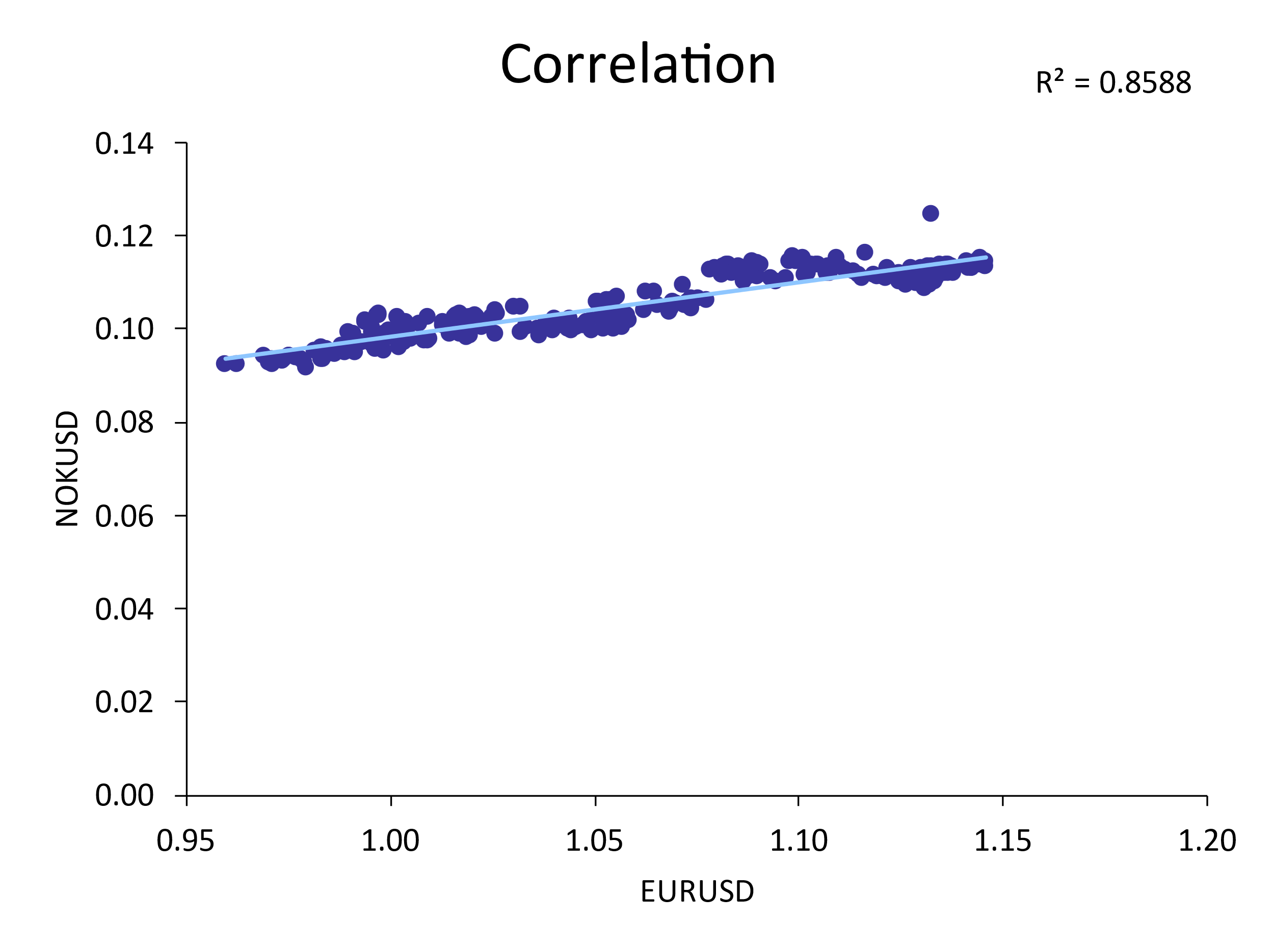
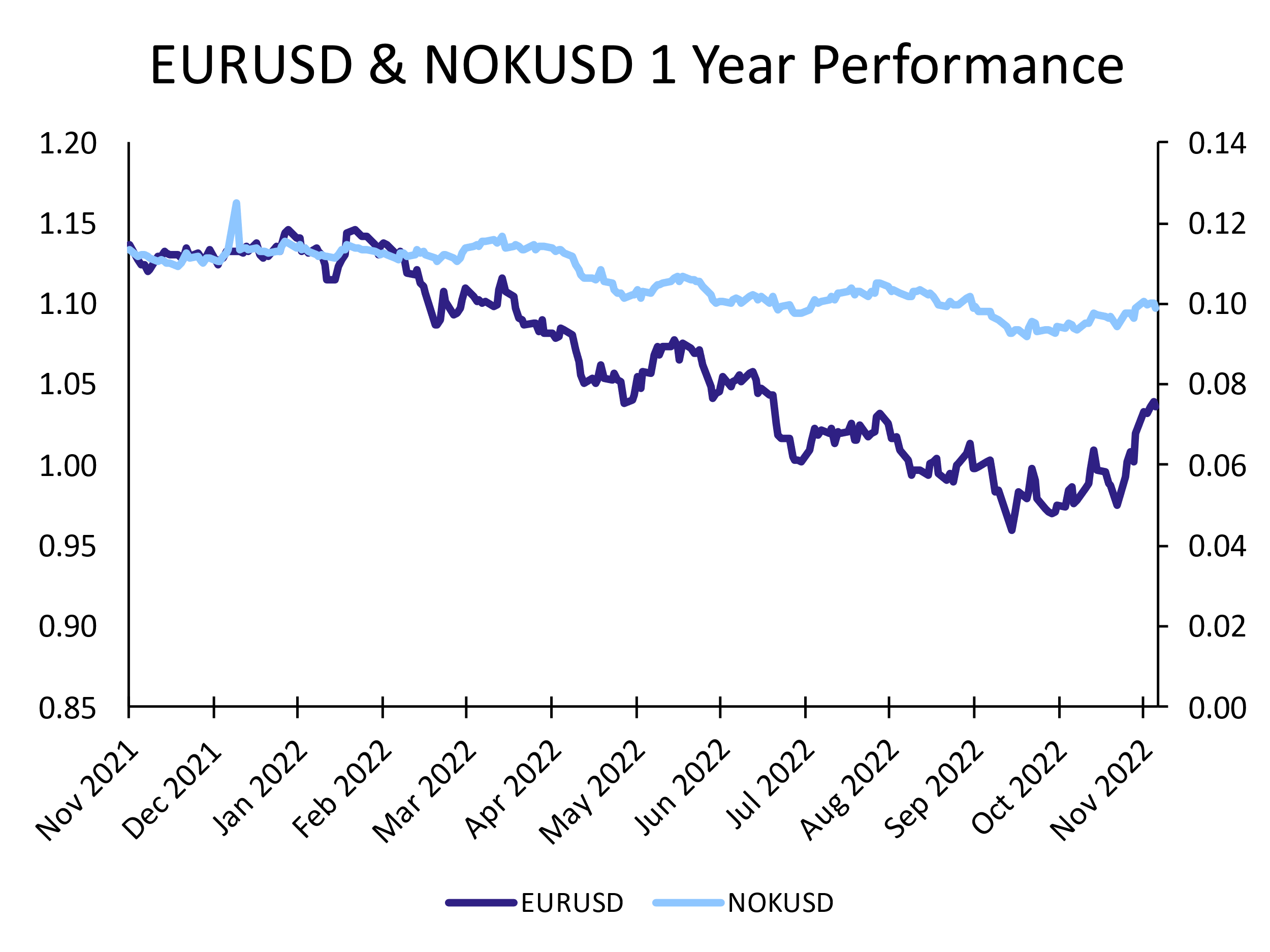
Source: Yahoo Finance, Bocconi Students Investment Club
Risks
Similar Inflation Growth in the Eurozone and Norway. Although inflation is currently slowing in Norway while remaining hot in the Eurozone, inflation readings have been difficult to predict in 2022. If inflation were to start moving in line (strengthening and weakening), the two central banks may implement policies that strengthen the correlation of the currencies.
Fed Accelerates Tightening. If the Fed has surprised the markets this year with the rate it has hiked interest rates. If it were to tighten rates aggressively and further outpace the ECB and Norges Bank, both currencies could see weakening against the US dollar, driving correlations between the two.


0 Comments