Introduction
Trading strategies revolve around several sources of edge, ranging from discretionary macro ideas, fundamental based stock picking to more sophisticated ones such as factors exposure or high-frequency algorithms. One area which the current literature pays little attention to is sentiment trading, which can be established in several ways. In this article, we explore an academic paper [1] that focuses its attention on Google Trends search volume data, providing trading signals for individual stocks in the S&P 500, considered underpriced according to retail investor sentiment. The authors backtest the strategy from 2004 to October 2014, thus we are performing a continuation of this backtest for the past 10 years. We will focus our work on an equally-weighted strategy with weekly-rebalancing, performing robustness checks as well as a factor regression to detect abnormal returns generated by it. We will then analyse the changes encountered when switching to a longer rebalancing period of one month. Lastly, we will present a different portfolio weighting scheme than the one used by the paper and explain our findings.
Methodology
Our work starts by defining the trading universe. According to the paper studied, there are 122 liquid stocks in the S&P 500 index which have enough search data provided by Google Trends. As a proxy for liquidity and due to time constraints, we focused on the first 122 stocks ranked by current market cap. Out of them, we found 82 of them with available data, for which we manually imported individual weekly search data, for two sub-periods of 5 years. This is the maximum period allowed by Google Trends in order to get weekly data.
There are two aspects worth mentioning here. First, the most efficient way as provided by the current literature to get accurate search results is by typing the firm’s name followed by the word “stock” in the navigator. This can be easily explained by the fact that people might search for Citigroup or Netflix due to pure interest in banking services or watching movies. Secondly, instead of showing the actual number of searches, Google provides a scaled score (GSV), ranging from 0 to 100, with 100 representing the maximum search volume over the selected period. This way, the strategy is based upon a relative measure rather than an absolute one. To get our signal, we will compare the current week’s score to the median of the past 8 weeks, by calculating the abnormal search volume (ASV) according to the following formula:

We distinguish between two different strategies. The “Main” one enters long a stock on Monday’s open price if past week’s ASV score is negative, indicating abnormally low attention. The “Loser” strategy requires past week’s return of the stock to be negative as an additional condition, which indicates an increased probability of under-pricing. In the first phase, both strategies equally-weight each stock in the tradable universe weekly.
Strategy Results & Robustness Checks
In this section, we are calculating the Sharpe Ratio (SR) of our strategy and its market outperformance, after running the backtest for two sub-periods, April 2015 to March 2020 and April 2020 to March 2025. By doing this split, we will be able to compare the performance between two different macro regimes, the low-rates environment and the post-COVID period.
In addition, we apply a t-test on the average weekly portfolio returns to check if the results are statistically different from 0, then we check the stationarity of our returns time series by using an Augmented Dickey-Fuller test and lastly, we correct for heteroskedasticity and autocorrelation of returns by applying Newey-West standard errors.
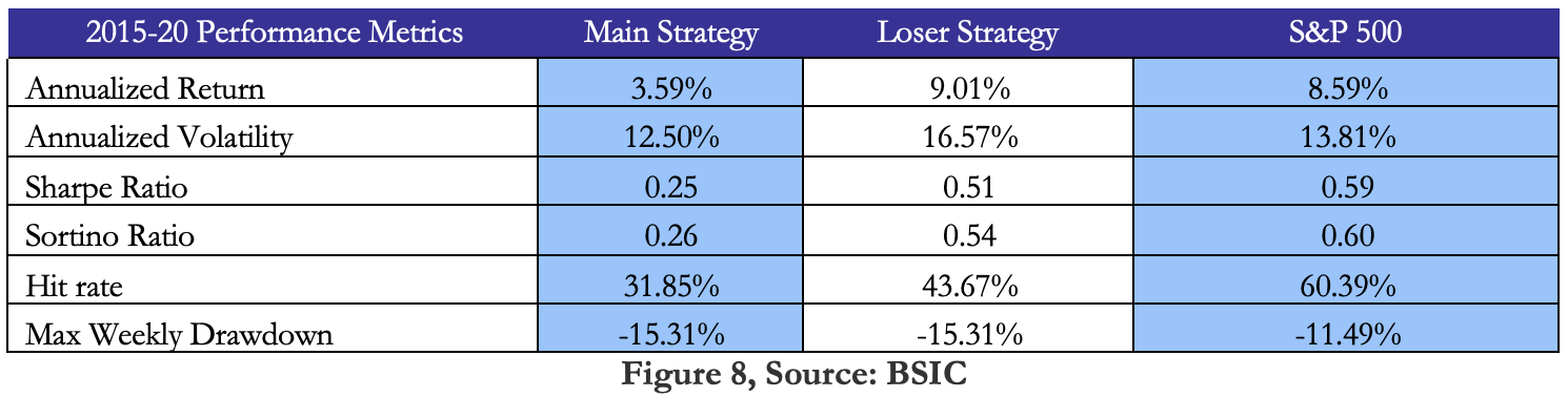
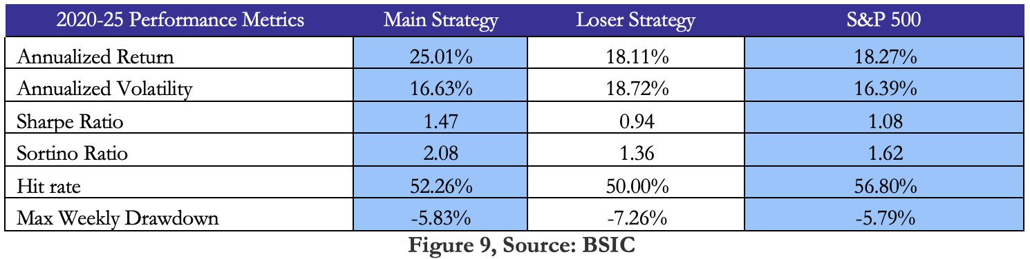
The returns series for both strategies and periods are significantly different from 0 and stationary. However, none of the excess returns relative to the market benchmark are statistically significant. Compared to the 2004-2014 period studied in the paper, this can be attributed to improved S&P 500 returns. Visual results can be seen in Figure 3 below, with very similar charts for the Main and Loser strategies.
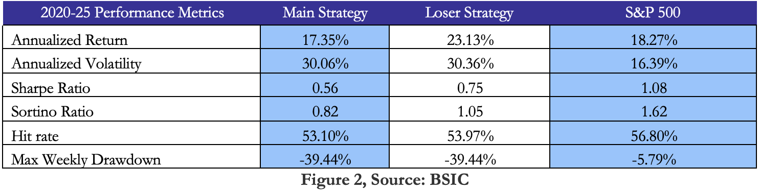
The most relevant performance metrics are shown in the tables above. As can be noticed, the only improvement in risk-adjusted returns relative to the benchmark comes from the Main strategy in the first sub-period analyzed and it is marginal. For a risk-loving investor, the Loser strategy in the second sub-period also delivers impressive returns, but with the caveat of significant drawdowns.
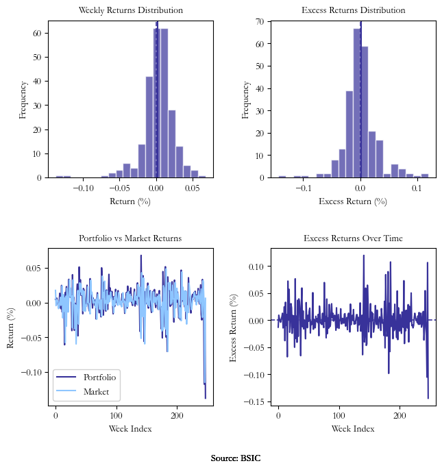

Figure 3, Left: Main Strategy, Right: Loser Strategy, Source: BSIC
Factor Analysis
The last step of our analysis consists in a factor OLS regression in order to check if the abnormal returns (alpha) are statistically significant for the two sub-periods. We have used WRDS to import the three Fama-French factors, the risk-free rate and the Carhart momentum factor. The equation used for our linear regression is:

where  is portfolio’s return,
  is the risk-free rate,
  is the intercept of the regression,
  is the excess market return,
  is the return of the “high minus low” portfolio,
  is the return of the “small minus big” portfolio,
  is the return of the “up minus down” portfolio,
  is the residual term and
  and
and  are regression’s betas.
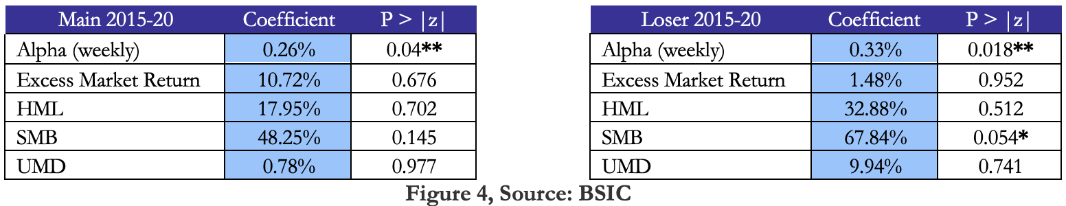
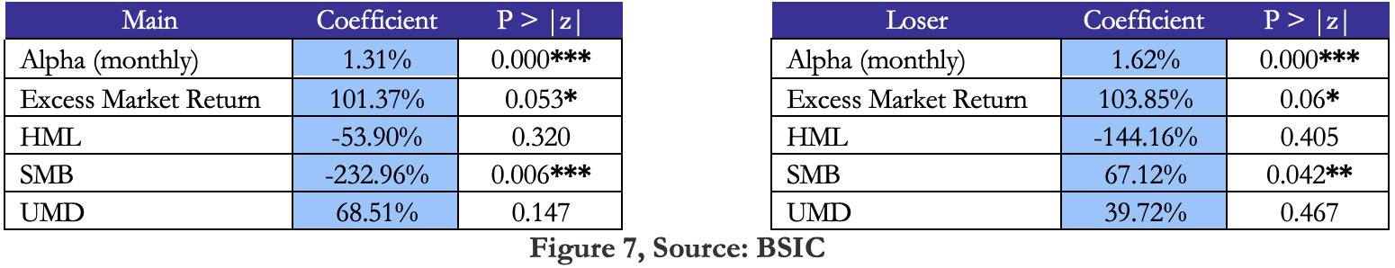
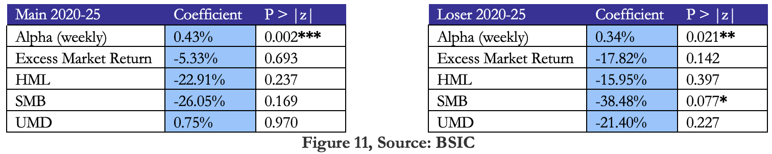
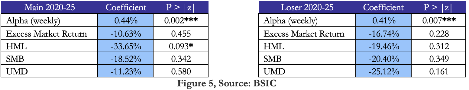 As noticed above, alphas are statistically significant for both periods and both variations of the strategy, with annualized abnormal returns ranging from 13.52% to 22.88%. The exposure to the factors used is nonetheless insignificant, with marginal exceptions for the SMB of the Loser strategy between 2015 and 2020, and the HML of the Main strategy between 2020 and 2025. So far, the results are consistent with the current literature’s findings.
Monthly Rebalancing
In this part, we continue our analysis by rebalancing the strategy monthly. Consequently, we will use monthly search scores for the entire period considered. The ASV is calculated similarly using the following formula:

This helps reduce transaction costs and allows us to inspect the effect of under-pricings as indicated by the search volume data on a slightly longer time horizon than weekly. Same as before, we will differentiate between the Main and Loser strategies and calculate performance metrics and conduct factor analysis, which can be found below.

The Sharpe and Sortino ratios are clearly improved relative to the weekly rebalancing, mostly due to significant reduction in the volatility of the strategy. It can indicate some randomness present in the weekly signal, as well as the fact that short-term movements are mostly dictated by institutional investors. At the same time, retail investors usually seek medium to long-term returns when looking for potential stocks to add in their portfolios.
The alphas are once again statistically significant, as expected, providing annualized abnormal returns of 15.72% and 19.44% for the Main, respectively Loser strategy. However, for this rebalancing horizon, the strategy also has statistically significant exposure to the SMB factor, a potential indication of the size effect being present in investors’ decision process.
A different Approach to Portfolio Weighting
Lastly, we tried implementing a new method of allocating weights to the individual stocks with a negative ASV signal. Instead of the original equally-weighted strategy with weekly rebalancing, we decided to allocate more the more negative each stock’s score is. Each week, for each stock i with a negative ASV score, its weight is calculated by the formula:

where the denominator represents the sum of absolute values of negative ASV scores in that week. In addition, we normalize each weight by the stock’s realized volatility and rescale the normalized weights such that they add up to 1. We do this in order to limit the returns’ exposure to factors other than the sentiment idea discussed in the introduction. By performing the same analyses as before, we acknowledge that this weighting scheme performs very poorly in the first sub-period, but it produces similar results to the equal-weighted one between 2020 and 2025.

In the 2015-20 period, returns are not statistically different from zero and neither are the alphas statistically significant. However, the picture changes for the second sub-period, with performance metrics significantly improved compared to the equally-weighted strategy, making the Main strategy an attractive alternative to the benchmark. The annualized abnormal returns are high enough at 22.36% and 17.68% for the Main and Loser strategies, once again statistically significant.
We tried implementing just the relative weighting method, without volatility normalization, however, the performance metrics were much worse.
To get a visual understanding of the difference between the two weighting schemes, we have attached below the cumulative performance charts of the 4 strategies versus the benchmark, for both sub-periods.

Figure 12, Period: 2015-2020, Source: BSIC

Figure 13, Period: 2020-2025, Source: BSIC
Accounting for Transaction Costs
The above results would be purposeless without a rigorous analysis of strategy’s transaction costs. When buying the security, the difference between ask and mid price is paid by the investor, while the difference between bid and mid price is paid when selling it. For simplicity, we will assume the transaction costs calculated in the paper as our baseline, which should hold true given market makers have grown more competitive over the past 10 years. As our tradable universe consists of about two thirds of the stocks used in the paper, the assumed transaction costs are about 0.0702% from returns for every single rebalancing period. That would account for an annualized 3.65% TCs for the weekly-rebalancing equal-weighted strategy and 0.84% TCs for the monthly-rebalancing equal-weighted strategy, both figures being significantly below strategies’ returns. The transaction costs for the relatively-weighted strategy cannot be precisely calculated, but they surely make the strategy worse off in the 2015-20 sub-period and are not great enough to counterbalance the impressive results obtained in the second half of our study.
Conclusion
In this paper, we aimed to provide the reader with a basic understanding of how a simple mechanism like Google Trends can serve as trade idea generator. We presented two versions of the signal required to enter the strategy, two rebalancing methods and two approaches to portfolio weighting. Further areas of research can include dynamic rebalancing based on the macroeconomic regime, inclusion of the VIX index as an additional signal as suggested by the paper, inclusion of more sentiment proxies or more systematic portfolio weighting methods.
References
[1] Storms K., Kapraun J. & Rudolf M., “In Search of Alpha – trading on limited Investor Attention”, 2015
[2] Storms K., Kapraun J. & Rudolf M., “Can Retail Investor Attention enhance Market Efficiency? Insights from Search Engine Data”, 2015
[3] Fang L.H. & Peress L., “Media Coverage and the Cross-Section of Stock Returns”, 2009
[4] Barber B.M. & Odean T., “All That Glitters: The Effect of Attention and News on the Buying Behavior of Individual and Institutional Investors”, 2008
[5] www.google.com/trends


0 Comments