Introduction
Natural language processing has recently become a tool with great applications in finance. Companies like JPM, Deutsche Bank, Statestreet are using NLP software to extract alternative data such as social media platforms sentiment, extract key insights from research reports and even flag possible executive deception by analyzing the earning call transcripts.
In this paper, we will apply NLP methods to sentiment analysis, by classifying the tweets of Elon Musk into three categories: positive, negative and neutral. The goal of this research experiment is to test if there is any predictability between the sentiment of Musk’s past tweets and Tesla’s daily stock price via Granger causality and then build a strategy on top of 3 sentiment signals derived from the tweets’ sentiment.
Past literature
To start with, numerous methodologies and conclusions have been drawn in the past in the field of behavioral finance, with a particular emphasis on the influence of social media sentiment on stock market dynamics. One of the earliest studies [1] concentrated on Yahoo! message boards and how they affected stock results. They found that sentiment had a small impact on the performance of individual stocks, but for the Morgan Stanley Technology index, they found a strong association. Another study in this field [2] aimed at predicting the direction of the stock market using dictionary-based sentiment analysis on Twitter data. Their results suggest that certain moods taken from Twitter could Granger-cause movements in the Dow Jones, indicating a strong correlation between public sentiment and stock market values. On the other hand another report [3] found that there are three ways to examine how social media affects the stock market: discussion volume, message content richness, and user popularity and competence. According to this theory, increased engagement on online platforms is correlated positively with greater stock trading activity.
Our study differs from these past approaches, as our model uses a transformer based model known as RoBerta to classify the sentiment expressed in a Tweet. This methodology provides a more accurate and detailed evaluation in contrast to previous, less complex methods that relied on dictionaries, such as Harvard IV-4 Psychological Dictionary for sentiment analysis, and OpinionFinder and the Google Profile of Mood States to evaluate public mood. Also, our focus lies on specifically analysing only tweets related to Tesla, a company we selected because of its widespread retail following, market volatility and a very active insider on Twitter, the CEO Elon Musk. Also, we use Granger causality tests to thoroughly investigate the ability of past sentiment to forecast fluctuations in the current stock price, going beyond the usual correlation analysis seen in past works.
Data Collection
For the research we conducted we had to use two datasets. We first found a dataframe containing Elon Musk’s tweets and likes received between 2010 and 2022 from an existing dataset and then collected data on Tesla’s adjusted closing stock price the same period for a daily frequency. In order to guarantee that we only included the most relevant tweets, we scrapped Tesla’s wikipedia page to come up with the most frequent words associated with Tesla, such as “tesla”: 396, “model”: 115, “company”: 90, “vehicles”: 71, “musk”: 56, ”battery”: 48. With this in mind, we focused on the following filtering words: “Tesla”, “Battery”, “Model S”, “Model X”, “Model 3”, “Cyber Truck”, “Roadster”, and “Semi Truck”. After doing this operation, we found that among Elon’s 17k tweets between 2010 and 2022 only 3k were relevant for our Tesla sentiment analysis, and classified the 3k tweets into negative, positive and neutral.
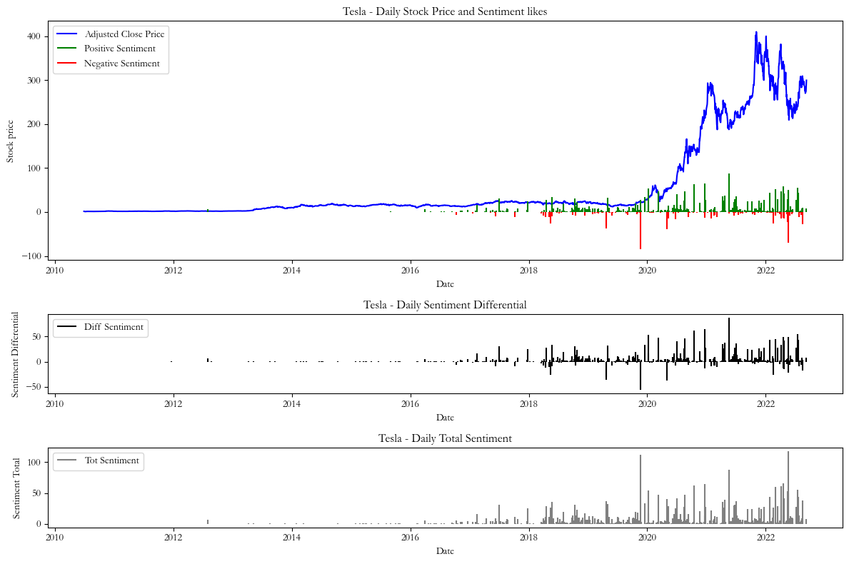
However, after removing the neutral sentiments from the dataset and plotting the total of positive and negatively labeled sentiments (as shown by the gray series in Charts 1,2 & 3) we realized that sentiment data was most frequent between 2018 and 2022, hence we only focused on this period.
Sentiment Classification
To classify the tweets with their corresponding sentiment we used the RoBERTa (Robustly Optimized Bert Pretraining Approach) model. This model is an advanced version of the BERT architecture, designed to deliver superior and more nuanced performance in tasks, such as sentiment classification.
BERT
First introduced by Google in 2018, BERT (Bidirectional Encoder Representations from Transformers) represents a significant advancement in natural language processing (NLP) with its bidirectional reading capability, which contrasts with the unidirectional approach of traditional models like recurrent neural networks (RNNs) and long short-term memory (LSTM) networks. Unlike its predecessors, BERT can comprehend ambiguous language by considering both left-to-right and right-to-left contexts simultaneously, thanks to its transformer architecture. While BERT was pre-trained on Wikipedia texts, it can be fine-tuned with question-and-answer datasets. Traditionally, BERT has been trained on two tasks: masked language modelling (MLM) for predicting masked words based on context, and next sentence prediction (NSP) for discerning logical connections between two given sentences. However, BERT can also be trained and used as well for downstream tasks such as sentiment classification.
RoBERTa
RoBERTa (Robustly optimised BERT approach) surpasses BERT through multiple advancements. It leverages a more extensive range of pre-training data, including datasets from BookCorpus, CC-News, Common Crawl, and Wikipedia, leading to richer linguistic representations. Additionally, RoBERTa extends training durations and batch sizes, capturing subtler language patterns and relationships. Unlike BERT’s static masking, RoBERTa employs dynamic masking, enhancing model robustness by masking different token subsets in each epoch. By omitting the next sentence prediction (NSP) task during pre-training and employing larger training steps, RoBERTa optimises its training process for better performance on downstream tasks. These collective improvements enable RoBERTa to outperform BERT across various natural language processing (NLP) tasks.
Applying RoBERTa
To classify the tweets we leveraged the deep learning capabilities of Hugging Face’s Transformer library by using a base RoBERTa model pre-trained on 124 million tweets to classify our tweets according to inferred sentiment: positive, negative and neutral. We apply the RoBERTa model only on Musk’s 3k Tesla relevant tweets and use the “yield” generator and batch processing so that we can process our large dataset without running out of RAM memory. A glimpse of our RoBERTa classified data can be seen in Table 1’s “sentiment” column. Also, as shown by the “Tesla relevant ” column the 3 rows shown are part of the 3k rows of data from our 3k Musk tweets that focus on Tesla Inc.
Table 1
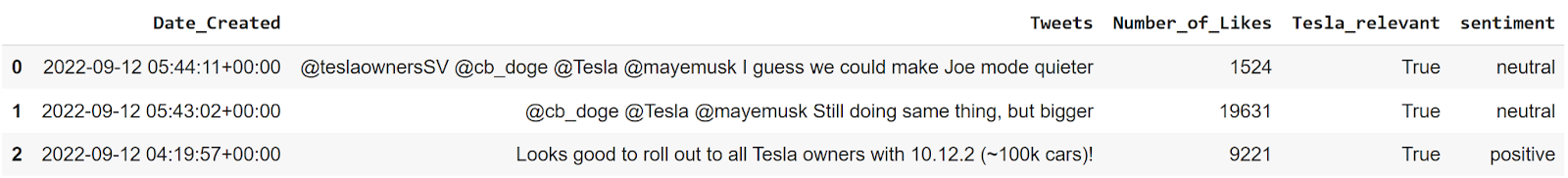
Source: BSIC, Kaggle
Signal Development
Our signal is based on the daily sentiment differential between the tweets which we classified as positive and negative, given that we excluded the neutral sentiments from our score. For our first signal (Chart 1) we calculate the daily sentiment frequency differential using the formula:

The second signal (Chart 2) modifies the previous formula by weighting the sentiment frequency by the total number of likes received by positive and negative tweets, according to the formula:

Lastly, the signal (Chart 3) takes the sum between the difference of total likes of positive and negative tweets in a day according to the formula:

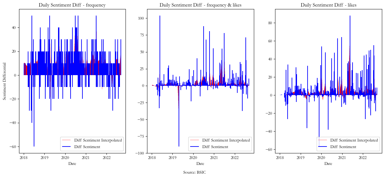
In the three graphs below we plot the resulting sentiments together with the stock price and obtain sentiment differential for each signal. We plotted the daily total of positive and negative tweets to justify our decision to focus on the data from 2018 to 2022, a timeframe with fewer gaps between the sentiment data that need to be estimated with interpolation.
Chart 1
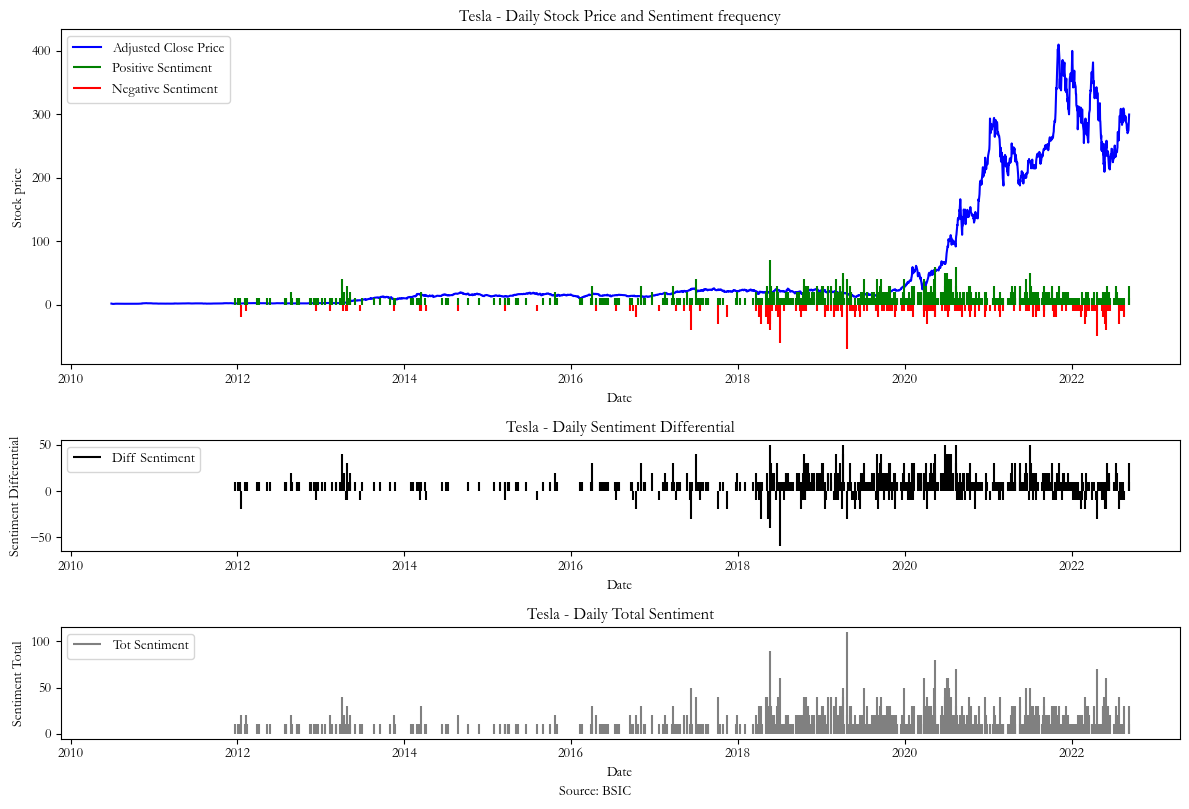
Chart 2
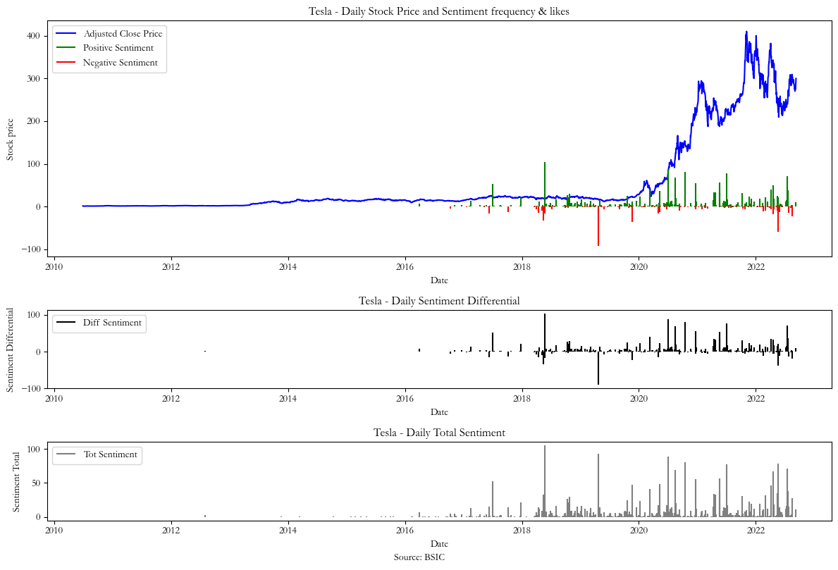
Chart 3
Interpolation
As it can be seen in the graphs 1,2 and 3 there are gaps in the Daily Sentiment Differential signal even after 2018 onwards. This is not due to lack of tweets, but rather because in our analysis we have excluded the neutral sentiment tweets by setting their value to zero. Hence we need to find a way to fill in the missing sentiment differential data, and to accomplish this we use spline interpolation. Spline interpolation [10] is a form of interpolation where the interpolant is a special type of piecewise polynomial called a spline. That is, instead of fitting a single, high-degree polynomial (in our case, a first degree polynomial) to all of the values at once, spline interpolation fits low-degree polynomials to small subsets of the values. Below, we show the interpolated data in red against existing data in blue for each of the 3 sentiment differential signals used, this way fixing the problem of missing sentiment data in certain days.
Stationary tests and transformation
Stationarity is a key concept relevant in time series analysis. A stationary time series is one whose statistical properties such as mean, variance, and autocorrelation structure do not change over time. There are two types of stationarity, strong and weak, and it is worth noting that in most academic contexts stationarity stands for weak weak stationarity. Without entering too much into details, a time series that has both its mean and covariance constant is called weakly stationary, while a time series for which all joint distributions are invariant to shifts in time is called strictly stationary.
As stationarity is an underlying assumption for correlation analysis, we need to make sure the series on which we run correlation tests are both stationary, and we do this via the Augumented Dicky Fuller test (which tests the presence of a unit root and hence lack of stationarity). Also, stationarity is required for our Granger causality tests, which would be unreliable otherwise. Consequently, after running the stationarity test for all the series considered: stock price, volume and sentiment scores we find that the only non-stationary data series is the stock price. To fix this, we decided to use log returns instead of stock price data as this is a form of differencing – the most popular way to make a time series stationary.
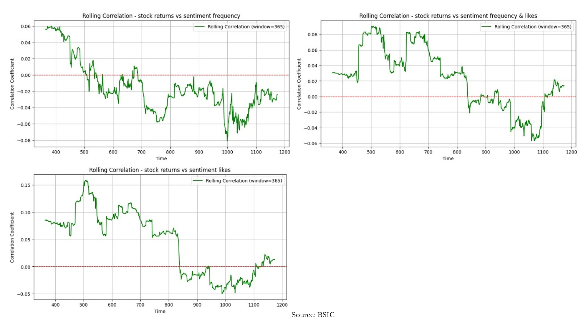
Correlation Analysis
Once we have made sure our data is stationary, we use correlation analysis to test the relationship between the sentiment frequency differential weighted and unweighted by likes with the tesla log returns. As previously mentioned, the period selected for the in depth analysis is between 2018 and 2022 due to the highest availability of sentiment data in this period, and consequently we have 4 years of daily stock returns and sentiments. However, instead of calculating the correlation between two series for the whole period, we chose to run a rolling correlation and plot it, in order to visualise the changing effect in correlation, but most importantly to make sure that the correlation between the series considered at the lag zero is close to zero. The low correlation between all three signals and the stock returns shown in the graphs below confirms that there is no instant incorporation of the sentiment into stock price.
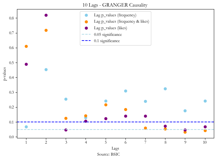
Granger Causality
Granger causality is a statistical test which assesses the predictability of the lags of a “causal” variable for the current values of the “effect” variable. It is important to mention that granger causality does not imply causality but rather the statistical significance of the lags of one series for predicting a second series. Empirically, we find that for signal 1,2 and 3 the significant lags at 5% are 1, 9 and respectively 3 & 9.
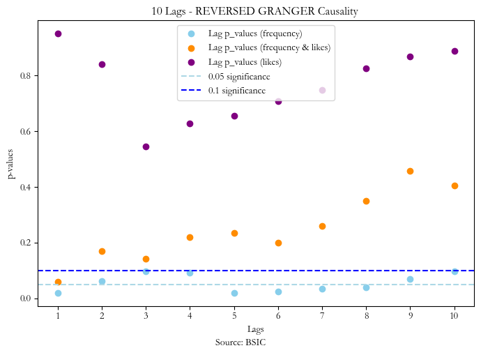
What is worrying is that the frequency of tweets seems to exhibit reverse causality at lag one too, which suggests that the frequency of positive over negative tweets of Elon musk are impacted by the stock price from the previous day. This should make us take any results of the first signal with a grain of salt.
Backtest & hyperparameter optimization
Using the sentiment analysis conducted by RoBERTa our trading strategy aims to execute daily trades both long and short based on the overall sentiment differential for all the 3 previously described signals.
To select the parameters for the three strategies we conducted hyperparameter optimization on the training set (2018 to 2020) to find the most optimal sentiment differential level for entering a long or short position, but also to find the best holding period, stop loss level and profit taking level. Using grid search, we consider a range of values for each hyperparameter and look to maximise the overall strategy’s return over a simple buy and hold strategy return, and then return the corresponding maximising parameter values. Using these parameters (Hyperparameters table), we apply each signal strategy to the test data (2020 to 2022). On each trading day our model checks if there is no position open and if the lagged sentiment signal went above the threshold for going long or short. It is important to note that for each we use the most statistically significant lag according to our Granger causality analysis for each sentiment signal to make our trade decision. Therefore, we trade on the assumption that the sentiment a few lags (days) back is not already priced in the stock. When a trade is opened, it stays open until we hit a take profit, stop loss or the pre-defined stop period.
Finally, to compute the total return of the strategy we sum the returns of the strategy corresponding with each signal and compare it with the buy and hold return for the period, a comparison that can be found in the results tables.
Hyperparameters Table
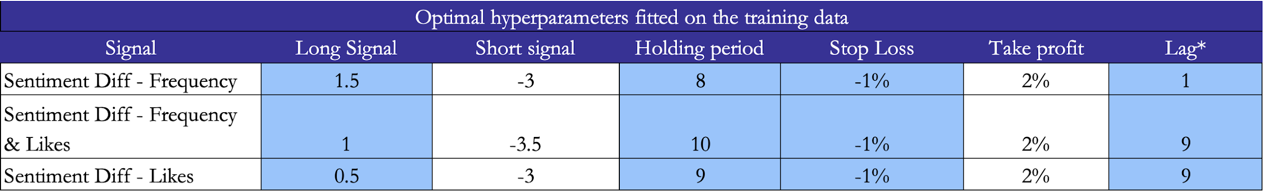 Source: BSIC (* Lag was not fitted with grid search, but it is the lag with the lowest Granger p-value)
Results Table
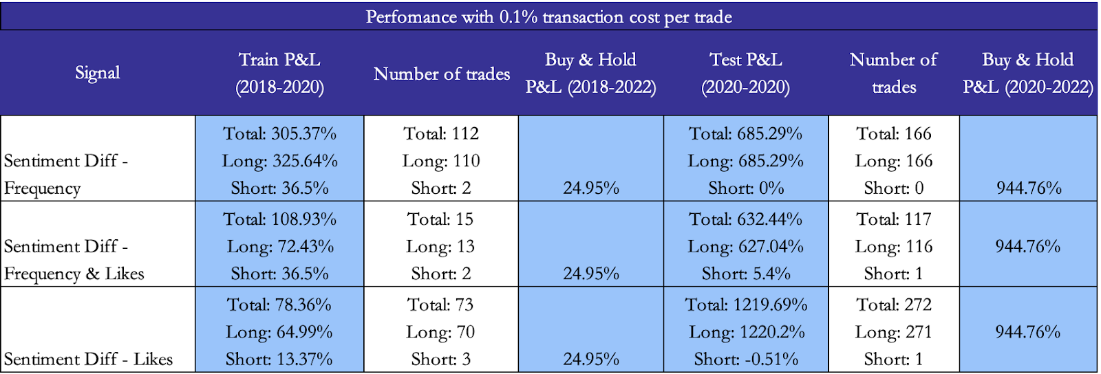 Source: BSIC
 Source: BSIC
Conclusion
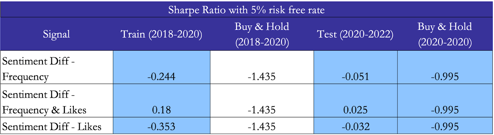
On the bright side, our results show that sentiment-based signals have some merit in regard to performance when used in tandem with hyperparameters such as the holding period, stop loss and profit taking levels optimised on a training set. What is surprising is the fact that all three sentiment signals exhibit a lower Sharpe ratio than the corresponding buy and hold strategies and even better, the Sharpe ratio improves in the test.
On the other hand, we notice that our Sharpe ratio is still negative for almost all scenarios, even though it is less negative than the Sharpe ratio of Tesla’s returns. Lastly, one should not forget that two of the sentiment signals considered exhibit reversed Granger causality with the stock returns, hence one should use sentiment signals with a grain of salt and ideally together with other fundamental or quantitative signals.
References
[1] Das, Sanjiv and Chen, Mike “Yahoo! for Amazon: Sentiment Extraction from Small Talk on the Web”, 2007
[2] Bollen, Johan; Mao, Huina; and Zeng, Xiaojun “Twitter mood predicts the stock market”, 2011
[3] Benthaus, Jan and Beck, Roman “Social Media Sentiment and Stock Prices – An Event Study Analysis”, 2015
[4] CardiffNLP “Twitter RoBERTa-base for Sentiment Analysis”, 2021
[5] HuggingLearners “Twitter Dataset for Tesla Analysis”, 2021
[6] Gajare, Neel “All Elon Musk Tweets – 2022 Updated”, 2022
[7] Bagwan, Sabir “Elon Musk Tweets 2010-2022”, 2022
[8] Bhadkamkar, Amey and Bhattacharya, Sonali “Tesla Inc. Stock Prediction using Sentiment Analysis”, 2022
[9] Edman, Gustav and Weishaupt, Martin “Predicting Tesla Stock Return Using Twitter Data: An Intraday View on the Relation between Twitter Dimensions and the Tesla Stock Return”, 2022
[10] Yu.N. Subbotin, “Interpolating splines” Z. Cieselski (ed.) J. Musielak (ed.) , Approximation Theory , Reidel (1975) pp. 221–234


0 Comments