Modelling Transaction Costs and Market Impact

Download PDF

Introduction

Transaction costs are a critical component of trading strategies, as they can have a significant impact on returns. Institutional investors need to be able to accurately model transaction costs to make informed decisions in backtesting and optimising their strategies. In this article, we will explore the various ways in which transaction costs can be modelled, including explicit and implicit costs, and how they can be incorporated into trading strategies. We will also discuss the challenges of accurately estimating transaction costs and the importance of considering the impact of transaction costs on the performance of a strategy.

Different types of transaction costs

Transaction costs refer to the expenses incurred by buyers and sellers when conducting a financial transaction. In the economic literature, these costs are represented as premiums paid above decision prices for buys, and discounts offered below decision prices for sells. Engle, Ferstenberg, and Russell (2012) estimated that NYSE stocks have an average transaction cost of 8.8 basis points (bps), while NASDAQ stocks have an average transaction cost of 13.8 bps.

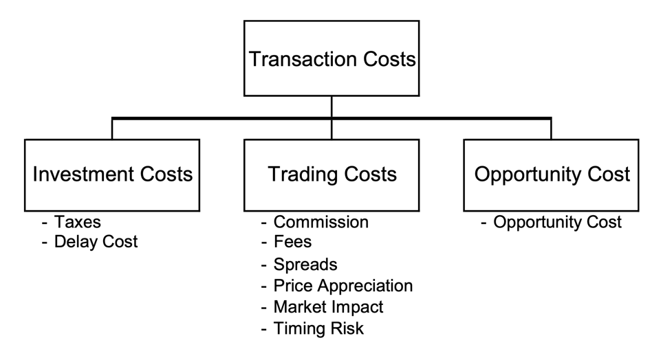
Transaction costs can be further categorized into different components, including fixed and variable costs, as well as visible (transparent) and hidden (non-transparent) costs. Fixed costs are unavoidable and independent of market prices, while variable costs depend on market prices and can be managed through implementation strategies. Visible costs are those components with cost structures easily observable from the market, such as commissions and taxes, while non-transparent costs are not market observable, such as market impact. Non-transparent transaction costs account for the lion’s share of total transaction costs and provide the greatest potential for performance enhancement. An image illustrating the most common costs to be considered is provided below.

It is worth noting that different markets offer various types of costs to look at based on the size of the trade. While the most common approach is to analyse the costs through an increasing slope as a function of trade size, which is typical for electronic, liquid equity and futures markets, other cases abound. For example, market impact may not be a fundamental variable when dealing with constant transaction cost (as a function of trade size) where the market has a large tick size and commission fees. In another corner scenario, for over-the-counter (OTC) markets, percentage transaction costs in these markets tend to be larger for small orders than for large orders, as it takes the dealer roughly the same amount of time to execute a small order from a retail investor and a large order from an institutional investor.

Transaction costs can become fairly complex depending upon trading region, asset class, volume traded and many more parameters. Even in addition to the broker’s own fees, there may be regionally specific and esoteric taxes that need to be paid, such as the UK Stamp Duty on share transactions. It is important for equity investors to have a comprehensive understanding of the major costs that they need to pay depending on the exchange and geographical location.

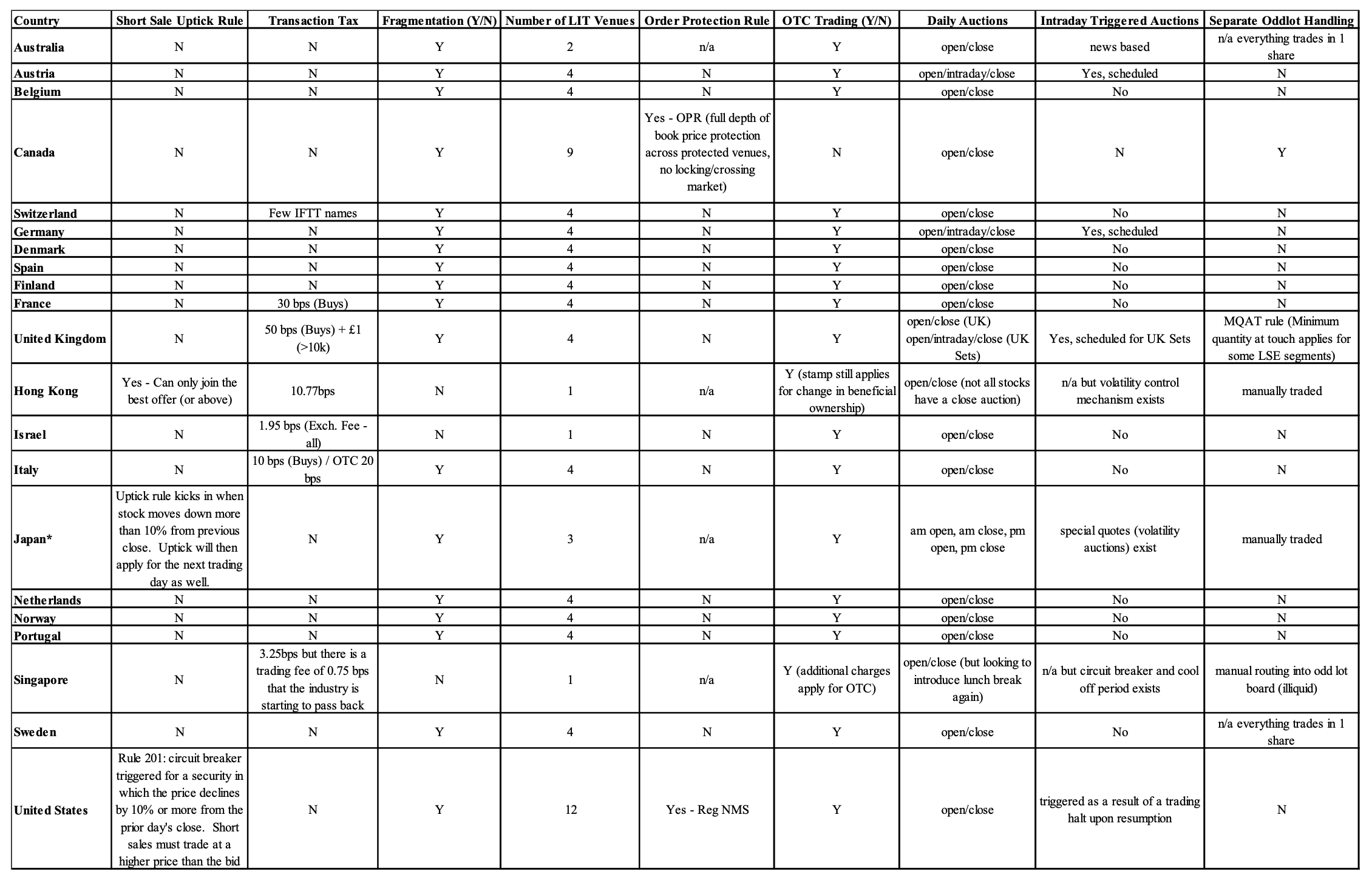
Different electronic exchanges and their costs
Source: Frazzini, Israel, Moskowitz (2017)

To fully measure quantitatively transaction costs, we can consider three central measures: the effective cost, the realized cost, and the cost relative to the volume-weighted average price (VWAP). The effective cost represents the difference between the price paid during the execution (on average) and the market mid-price before the trade happens. The realized cost, as the second term of the difference, has the mid-price at some time after you stop trading, say after 5 minutes when prices have stabilized again. If your order has a long-lasting price impact, then the effective cost is larger than the realized cost. Finally, the cost relative to the VWAP is compared against the volume-weighted average price. However, note that this final measure is inappropriate in case of order book imbalances, such as a single buyer/seller in the market throughout the day. Indeed, in such a scenario TC(VWAP) = 0 even if we clearly incurred in transaction costs.

When considering all the measures for trading cost, we need to be wary of the way that the trading pattern changes in the real world given our constraints. From an economic theory perspective, opportunity cost represents the foregone profit or loss resulting from not being able to fully execute the order within the allotted time period and is measured as the number of unexecuted shares multiplied by the price change over the period the order was in the market. A core concept in this setting is the implementation shortfall, which can be described by two formulas: (1) the cost of execution relative to the arrival price, and (2) the sum of the opportunity cost and the cost of execution relative to the implementation shortfall benchmark.

IS = Trading Costs + Opportunity Cost = real performance portfolio – paper performance portfolio

Where, rather than explicitly computing IS, it is of paramount importance for money managers to see whether to focus the alpha research process on improving the trading implementation or the strategy’s alpha signals. Trading faster implies that the transaction costs rise but the opportunity costs decline, while trading more patiently shows that transaction costs drop but the opportunity costs rise.

Other costs: funding a strategy

One of the key differences between paper trading and live real trading lies in the fact that real-world portfolio management requires funding, and liquidity risk plays a crucial role in the day-to-day workings of any money manager. In order to leverage long positions, hedge funds typically borrow using securities as collateral. These loans are provided by prime brokers or repo lenders, and they appear on the liability side of the hedge fund’s balance sheet. To further support margin requirements for long positions, hedge funds may also utilize their own equity capital.

On the other hand, when a hedge fund sells securities short, they are taking on a liability, as they will eventually need to return these shares. The cash proceeds from the sale are still considered assets, although they are held as collateral by the securities lender. The securities lender may require additional cash as margin requirement, which means that the hedge fund must use its own equity capital to support margin requirements for short positions. To further mitigate risk, hedge funds often have additional equity invested in cash instruments such as money market funds, Treasury bills, or margin excess with prime brokers, which can help them sustain losses without immediately having to liquidate positions.

When estimating the margin needed for leveraged long positions, brokers will often use value-at-risk (VaR) and stress tests. A good approximation for a long position is one where the probability of a price drop greater than the margin requirement is low, typically below 1% or 5% over a short timeframe of 5-10 days. It is important for money managers to closely monitor their margin requirements and ensure that they have adequate funding and liquidity to support their investment strategies. For instance, recent computations show that a portfolio comprised of the S&P 500 has a 5% VaR over a 1-month horizon of 8.59%.

If a hedge fund takes a short position, its broker will be afraid that the hedge fund will fail when the price goes up: if the fund fails to buy back the borrowed shares, the broker needs to do so. Since the broker has the sale proceeds as well as the margin requirement, the broker can do this without using its own money, as long as the current price P(t+1) is no greater than the sum of the sale proceeds and the margin, P(t) + m × P(t).

Each day, a hedge fund’s positions are marked to market, meaning that the value of each security is reassessed. The Profit & Loss profile is thus as follows:

Where the financing can be broken down to the cost of the cash loan from the prime broker to support long positions, the interest earned on the cash collateral held by the securities lender, and the interest earned on the additional cash in money market products:

Note that, while Prime Brokerages sometimes try to let the margin requirement depend on the overall portfolio (i.e. cross-margining), every day the cash account situation needs to be monitored in the case of a margin call. This is especially important with derivatives that have an embedded leverage but may start with a market value of zero.

As a final point, market impact is often incorrectly referred to as slippage or erosion. While it does constitute a part of these terms, it certainty does not comprise the entire portion. Market impact costs will occur for two reasons: the liquidity demands of the investor and the information content of the order. Mathematically, the market impact cost of an order is the difference between the price trajectory of the stock with the order and the price trajectory that would have occurred had the order had not been released to the market. Unfortunately, it is not possible to construct a controlled experiment to simultaneously observe both circumstances of price evolution. Market impact has often been described as the Heisenberg uncertainty principal of finance and explored by a variety of different papers that we proceed to explain.

Empirical evidence from the literature

In the past, market microstructure models focused on a single factor, such as order processing, inventory control, or adverse selection, to determine the quoted price of a security. While this approach allowed for an in-depth analysis of each factor, in reality the bid-ask spread likely incorporates the effects of all these factors to some extent. In a study by Stoll (1989), it was found that the quoted spread indeed reflects all three factors and that the components of the bid-ask spread, as contributed by each factor, remain constant as a percentage of the quoted spread.

Around the same time, Roll (1984) introduced an effective spread measurement model that proved to be an appealing alternative in market microstructure. The model estimates an effective spread directly from time-series data of market prices, eliminating the need for recording and matching quoted and actual prices for a particular transaction. Based on the assumption that spreads consist of only order-processing costs, the model demonstrates that the presence of a bid-ask bounce, where orders are executed at bid and ask prices instead of the mid-quote, leads to negative serial autocorrelation in security returns.

Therefore, an effective spread can be calculated from the observed serial correlation of transaction prices, as follows:

Here, S is the spread, and is the serial covariance of price changes. Choi, Salandro, and Shastri (1988) extended Roll’s model, incorporating the probability of a transaction at a bid or ask following the previous transaction. We should also note that Roll’s computation do not differ far from the illiquidity proxy conjectured by Bao, Pan, and Jiang Wang (2011) and discussed in a our research paper here.

Following a first period of market microstructure models, possible ways to express the price impact function ensued. The first model is a structural model estimated from US equity data (Almgren et al. 2005), where the model for market impact on trading is given by:

where , γ = 0.314, η = 0.142, σ is the daily volatility of stock return i at the beginning of month t, is the total amount of shares outstanding in the security, is the average daily trading volume of the stock (shares traded), sign() is a function that is -1 if shares are being sold and 1 is shares are being bought, T is the time interval in which the trade takes place in number of days and represents the number of shares of the security the portfolio is trading. Subsequently, the Northfield model in 2009 has introduced a price impact with a square root function in trade size according to the formula:

where and are parameters estimated by Northfield, is the number of shares to be purchased for security i in month t, and is expressed in terms of percentage price movement. The approximation, according to Chincarini (2017), results satisfying with the fitted parameters of B = 0.0206, C = 0.5096, resulting in an .

Hence, the task of modelling the price impact function of a large trader has been a challenging aspect of the transaction costs literature for some time. However, recent research has presented a significant shift in the field, as new models have been introduced that estimate transaction costs at far lower amounts than previously assumed. One such study, “Trading Costs” by Frazzini, Israel, Moskowitz (2017), not only presents a new model but also challenges the accuracy of cost estimates that ignore price impact, such as those based solely on effective spreads. The study collects trading cost data from three different brokers (ITG, Deutsche Bank, and JP Morgan), and a consulting firm (ANcerno) who collectively cover trades from more than 2,000 institutions.

Despite the historical difficulty in accessing data on market impact costs, the authors of the AQR paper emphasize the importance of a good model that uses trade size as an input and is a good proxy for modelling the price impact curve. It is also important to note that the best-performing brokers may handle more difficult orders on average, which could skew their performance measures. Overall, the study provides a valuable contribution to the literature by offering new insights into the complexities of trading costs for large traders, since the authors access a unique dataset of over $1.7 trillion live executed trades from a large money manager from August 1998 to June 2016, across 21 developed equity markets.

The estimated price impact model is based on market conditions, stock characteristics and trade size calibrated to both U.S. and international live executed trades.

where = 100 × / is signed dollar volume (m) as a fraction (in %) of the stock’s average past one-year volume (). “buysell” is a variable that equals 1 for buys and -1 for sell, “time trend” a linear time trend data series to capture changes in aggregate trading costs over time due to technology, changes in tick size, while [log(1+ME)] includes the market value of the equity, as well as the stock’s one-year volatility and the value of the VIX.

The paper constructs long-short anomaly portfolios based on techniques documented in the literature (e.g., SMB, HML, UMD, etc.) and applies trading costs to these portfolios using live trading data. The estimate of market impact is just under 9 bps on average for all trades completed within a day, with around 85% of that price impact being permanent. In their sample of U.S. stocks, the authors find a median transaction cost of 4.9 bps and a weighted average of 9.5 bps, while the estimated transaction costs for global stocks are larger, with a median of 5.9 bps and a value-weighted average of 12.9 bps. Finally, the estimated transaction costs are lower for small trades than for large trades, with trades that constitute about 10% of the typical volume having estimated transaction costs of about 40 bps. The authors estimate a cost of $0.005 per share for commissions.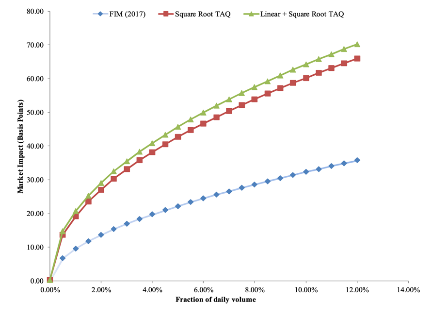

Average market impact curve (FIM 2017) compared to the previous models in the literature
Source: Frazzini, Israel, Moskowitz (2017)

As a final note, most money managers in the industry use third-party risk models to manage their portfolios. These models include MSCI-Barra, Northfield, and Axioma, with Barra having the largest market share at around 50%. These models are all multi-factor models, which means they assume asset returns can be represented as a linear combination of common risk factors. The Barra US Equity Model has been active since 1995, while Northfield’s US Fundamental Equity Risk Model has been active since 1990, and Axioma’s Robust Risk Model for the US has been active since 1982. Barra, for instance, uses four factors – volatility, elasticity, intensity, and shape that characterize a specific asset, one factor (market tone) that approximates overall market conditions and one factor (investor’s skill) that relates the forecast to a specific investor’s trading ability for estimating market impact costs.

A coding example in portfolio optimization

An interesting way to apply the concepts described so far about transaction costs is through modelling a portfolio selection problem which considers different possible transaction costs. To do so we use MOSEK Python library, which allows to translate into code and solve complex constrained optimization problems. We consider mainly two models: a market impact model as the impact on prices caused by the amounts we trade as liquidity at certain price levels is reduced; and a fixed and variable transaction costs model, which can take as inputs actual rates asked by exchanges to trade securities and that considers lower bound buy-in thresholds to avoid unrealistically small trades. We briefly introduce the mathematics behind the models, to then show an example of MOSEK models and their application on a set of stocks of the S&P 500.

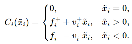
For the transaction cost model, we can consider two types of costs: fixed costs which are incurred regardless of the volume transacted, and variable costs that grow linearly with the volume traded. We can consider a different set of fixed and variables costs and respectively associated with buying and selling security i. Linear variable costs, for instance, are particularly useful to model costs related to bid/ask spreads, slippage, borrowing costs and shorting costs, as well as managing fees. Now let be the change in portfolio allocation. From this we can model our transaction cost function as a piecewise linear convex function:

By introducing two binary vectors we obtain an optimization problem as follows:

Where is the vector of expected returns, represent the upper bounds of amounts long/short of securities and ensure that if security i is traded (either being long or short) then transaction costs are incurred.

We can implement the following maximization problem into a python model. Firstly, we assume that . We also allow for shortselling, but we put an arbitrary threshold at a 30% portfolio size. We then define the variables, both their positive and negative part for x and the two binary vectors, constrained such that only either can be 1 at any given time (i.e. you can only buy or sell a security at any point in time):

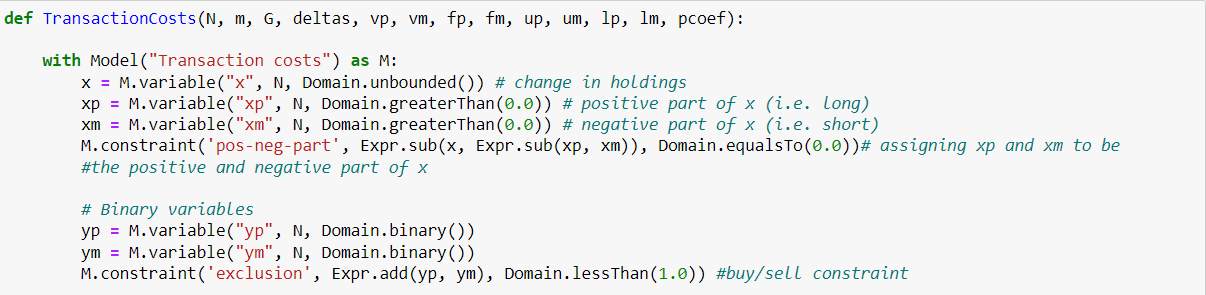
We can then add our budget constraint inputting our fixed and variable cost variables, as well as our max leverage constraint which is set at 130/30 in this example.

We can now apply the model to a variety of situations, for example to compute the efficient frontier of a set of stocks in the S&P 500. Considering the investment period from March 2018 to March 2023, we obtain the following efficient frontiers with and without transaction costs:

Source: Bocconi Students Investment Club

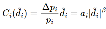
Market Impact model

As we already discussed, market impact represents the effect on the price of a security as a consequence of the volume we trade on the market: the larger the trade, the more relevant its market impact on the security, as we increase demand for that product, and we consume available liquidity. Mathematically, consider the dollar amount of our trade for security i to be Then for a security i of volatility we have that the change in price is:

Where is the average dollar volume in a unit period and are calibrated empirically. We can therefore express this in terms of our cost function as done previously for our transaction costs model:

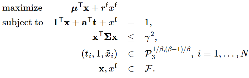
After normalizing by q to have the cost in terms of portfolio allocation we can use a constrained power cone: with . To avoid t from becoming excessively small, we can add a risk-free security to our investment universe so that the model allocates a correct amount to the risky security. The optimization problem therefore becomes:

To model market impact in python, we can use a regular Efficient frontier optimization model, adding the variable for our market impact and its constraint. Using the same stocks as before and the same investment period, we get the following result:

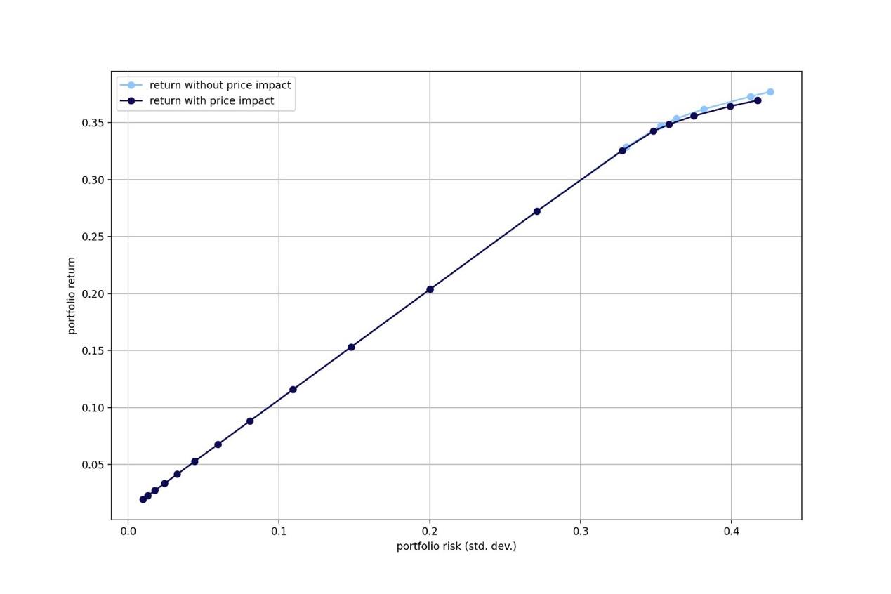
Source: Bocconi Students Investment Club

Conclusion

Modelling transaction costs is an essential component of designing and implementing profitable trading strategies. Traders must consider the impact of market liquidity, bid-ask spread, and market impact on the transaction costs of their strategies. They must also manage the capacity of their strategies, identify sources of funding, and understand the balance sheet of their hedge funds. By using the appropriate models and techniques for estimating transaction costs, portfolio managers can optimize their trading strategies and achieve better risk-adjusted returns.

Sources

• Engle, Ferstenberg, and Russell (2012), Measuring and Modeling Execution Cost and Risk
• Frazzini, Israel, Moskowitz (2017), Trading Costs
• Stoll (1989), Inferring the Components of the Bid-Ask Spread: Theory and Empirical Tests
• Roll (1984), A Simple Implicit Measure of the Effective Bid-Ask Spread in an Efficient Market
• Bao, Pan, and Jiang Wang (2011), The Illiquidity of Corporate Bonds
• Almgren et al. (2005), Direct Estimation of Equity Market Impact
• Chincarini (2017), An Approach to Enhanced Indexing