Introduction
In many financial studies the default assumption is that changes in prices are random and independent between different financial instruments. Opposing studies, thus, are often concerned with discovering dependencies and whether they are driven by common economic factors. One approach to the problem are network graphical models. With respect to finance theory, network graphical models appeared in the literature in 1999 and have been advanced since. Here, we want to delineate the pioneering methodologies in network modelling and give an example of a subsequent, more recent modification that tries to overcome some of the deficiencies of the early models.
Network graphical modelling is a powerful tool in addressing multivariate systems of uncertainty and complexity that can be formalized as a framework of connectivity. A subset of such systems is organized taxonomical where the individual elements can be segregated into clusters and subclusters that assume a specific interdependence. In this context, the systems’ complexity is dealt with by the respective procedures of clustering which are termed “filtering procedures”. As the term suggests, the procedures build upon dependence measures that describe a system’s elements as concise and complete as possible and filter them to retain only the significant dependencies of interest. In other words, the procedures try to single out key information by filtering a complex graph into a simpler relevant subgraph. It can already be suspected that under this formulation there is a discrepancy between the richness of retained information and system simplification, resulting in different approaches of balancing these two factors.
Among the network models, however, a distinction is often made between models that rely exclusively on Pearson’s correlation coefficient and models that deviate from such simplicity, e.g. models that are based on a more generalized version of correlation, broadly referred to as mutual information. Since the rather intuitive correlation-based models laid the foundation of network modelling in finance, we will concentrate on these in order to generally familiarize with the concept of network modelling in financial context, and present two recent concepts that build upon these correlation-based networks.
Correlation as the basis of network modelling
First and foremost, the correlation coefficient allows for the simultaneous investigation of observations of a multitude of variables, such as market return time series of several global indices. The crucial understanding which makes correlation of interest for network modelling in finance is that there is economic information stored in the correlation coefficient matrix. Then it is not surprising that the literature of network models with financial application started on the basis of correlation. The central importance that the correlation coefficient enjoys in the context of network graphical models, especially at the beginning but also in more recent literature, is rooted in the intuitive understanding of it as a similarity indicator and the straightforwardness of its transformation into a distance measure.
The possibly most cited publication which pioneered correlation-based network identification, both in terms of taxonomy as well as topology, is Mantegna’s (1999) “Hierarchical Structure in Financial Markets”. The motivation was to find a topological organization particularly of stocks (elements) in a portfolio (system) that may further explain the underlying common economic factors among these stocks. The innovative concept suggested in Mantegna (1999) is the transformation of correlation coefficients that allows for the definition of a Euclidean metric which in turn serves as a distance between the stocks in a portfolio. Correlation itself, however, cannot be used as a meaningful distance between two elements because it does not fulfil the three axioms that define a Euclidean metric.
The concept of distance between the two elements  and
and  , when observing their time series synchronously (no lag), is the following. Based on correlation, each system is defined completely by
  coefficients
  in a symmetric distance matrix
  which is a biased mirror image of the correlation matrix. The relationship between correlation coefficients and their associated metric distance is illustrated as follows
The distance is calculated according to the formula  , where
  is the correlation coefficient between element and . Then it must hold (i)
  if and only if
  , (ii)
  , and (iii)
  . Hence, the measure fulfils the three axioms of a Euclidean metric. Yet, for the filtering procedure that follows, the transformation of correlations into distances, axiom (iii) is modified to the stronger inequality
  , thereby taking on the hypothesis of an ultrametric space for the system. Ultrametric distance axiomatically expresses the association of the elements in a system as a hierarchical structure. In Mantegna (1999) and several other academic explorations, specifically the subdominant ultrametric structure is chosen by applying Kruskal’s algorithm for the construction of the network graph. This construction methodology leads to a minimum spanning tree (MST) of the system (see figure below). The MST is a graphical concept in which the n elements are linked by
  edges weighted by their distance, such that the sum of weights is minimized.
The construction of the MST by means of Kruskal’s algorithm extracts the upper (or lower) triangular part of the distance matrix , comprising elements, which are then sorted as an ascending sequence. The algorithm starts with the lowest distance and adds it as an edge between the two corresponding elements which mark nodes in the network, followed by sequentially adding further edges under the condition that they do not create cycles. Under this formulation,  marks the shortest distance from element to following a path in the MST.
Source: Bonanno et al. (2003).
An actual portfolio allocation algorithm that uses the MST is given by López de Prado (2017), known as hierarchical risk parity (HRP), which gives exact weights of allocation for a portfolio. The idea is that HRP finds a compromise between diversifying across the single assets and between clusters. The latter are given by the MST. Findings show that with a basic Markowitz portfolio allocation, the benefits of diversification are often more than offset by estimation errors. This leads to the fact that, on average, such portfolios fail to outperform out of sample, even compared to an equally weighted portfolio. By comparing Markowitz’s and equally weighted portfolios with HRP portfolios in random return simulations it was found that HRP provides both less common and less idiosyncratic shocks which resulted in reliably lower total portfolio variance out of sample.
A less intuitive but more recent multi-dimensional network methodology based on correlation is presented in Phoa (2013). The method is related to principle component analysis in that it uses eigenvectors and -values to breakdown the system and map its elements on a joint scale. More specifically, a new matrix  is computed based on the correlation matrix where
  . Then, each element
  is divided by the row sum to get the probability transition matrix
  . This is followed by the computation of the eigenvalues
  and eigenvectors
  of . Then each eigenvector defines a coordinate
  for each element
  . The diffusion map projects the elements in Euclidean space by defining their location based on the collection of coordinates as

The diffusion map is multi-dimensional, thus, to visualize the result, it is suggested to take the first two or three coordinates to plot them in a two- or three-dimensional space. With this method however, the coordinates do not have an intuitive economic meaning and only the distance between the elements is of relevance. This allows to measure the cloud of elements in the multi-dimensional space with respect to its dispersion, i.e. its portfolio concentration risk.
This rather abstract perspective on networks provides a methodology which, instead of focusing on the computation of distances, mediately extracts coordinates in a multi-dimensional space. The procedure leads to a diffusion map allowing to measure portfolio concentration risk. The diffusion map for monthly stock returns of the S&P 100 index between January 2002 and April 2012 as well as of the S&P 500 between July 2003 and April 2012 is subsequently investigating, the prior of which is illustrated in the figures below for the first three eigenvectors. As is the case for principle component analysis, the eigenvector decomposition presents the orthogonal factors with decreasing explanatory power. Thus, it is reasonable to concentrate primarily on the first three.
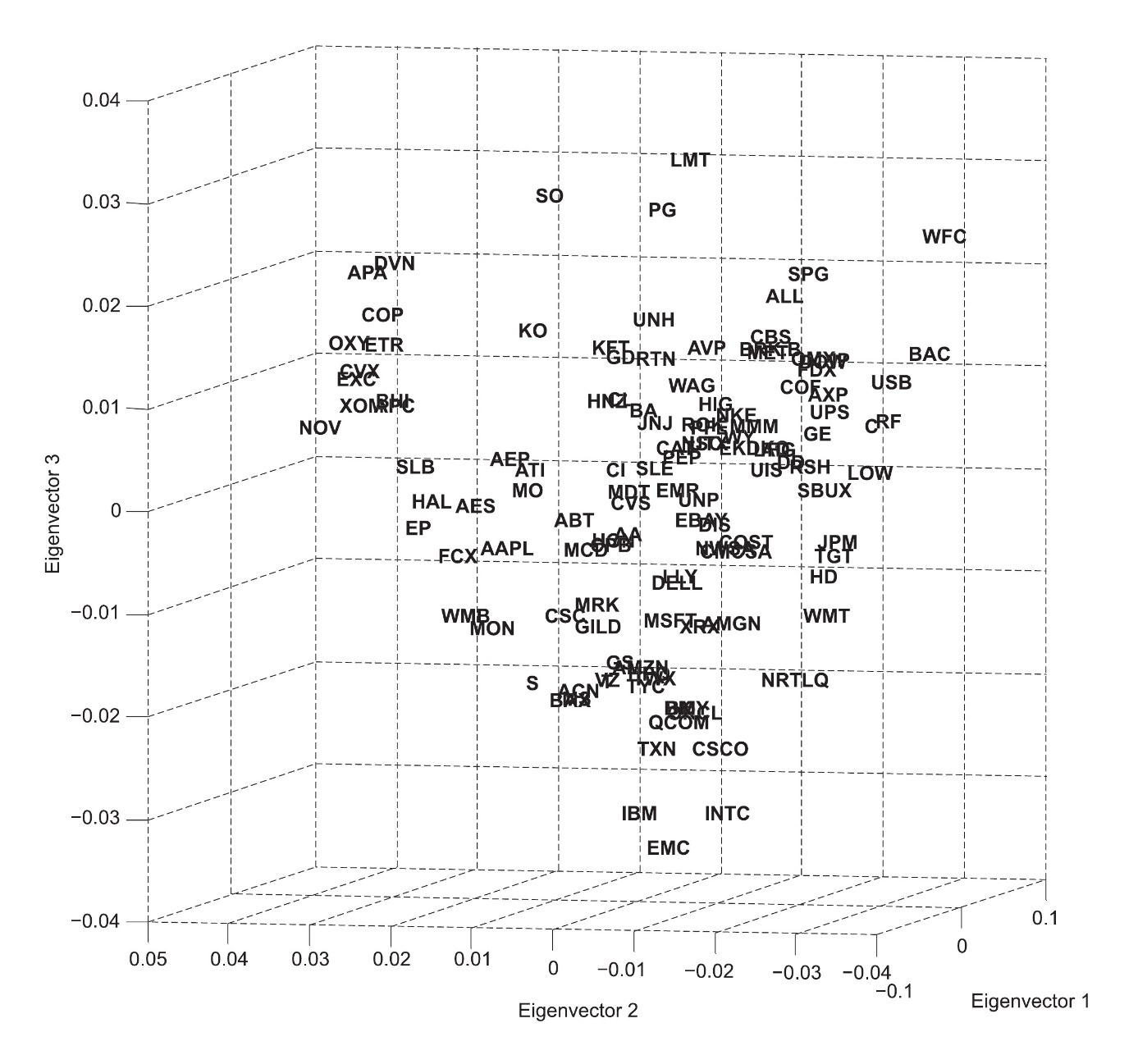
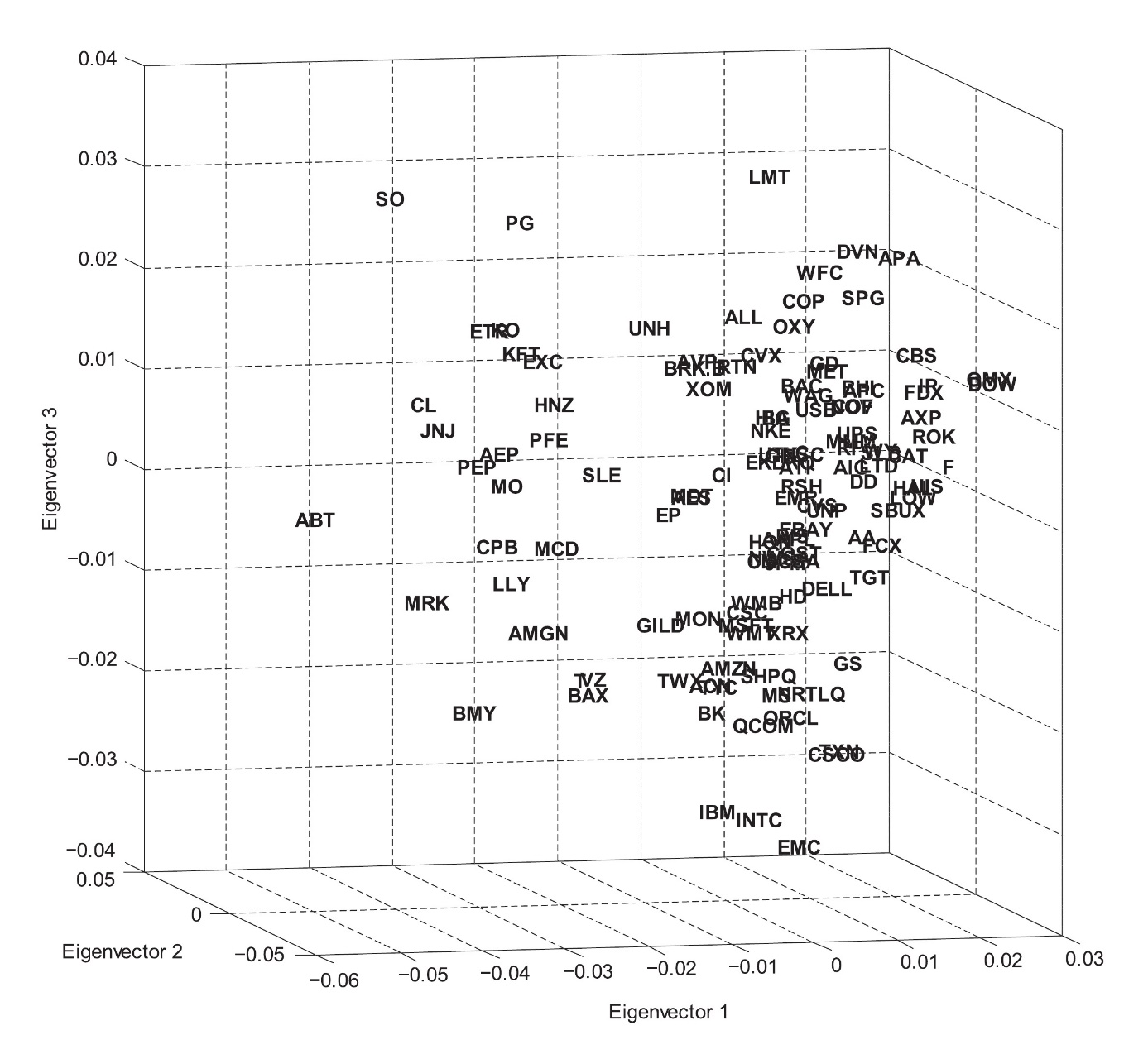
Source: Phoa (2013).
The diffusion map depicts the  elements of a system in a multi-dimensional space, possibly up to dimensions. For a better conveyance of the structure the diffusion map is shown with eigenvector 2 on the abscissa and eigenvector 1 on the applicate (top) as well as reversed (bottom).
It is argued that the extend of dispersion in the diffusion map provides information about the diversification across the portfolio. Thus, a global concentration measure can be defined that corresponds to the weighted covariance of the elements’ coordinates. Applied to the S&P 500 over rolling 12-months periods, it can be found that the global concentration gradually declined during times of economic stability and that it rose sharply during the financial crisis in 2007. After a following drop of concentration in 2008 and 2009 another sharp increase is observable during the equity rally in 2010.
The diffusion map methodology is particularly interesting when studied for its ability to stress test the network for idiosyncratic shocks. Define a local shock as a symmetrical normal density function, rescaled to have unit maximum, that has its peak at the coordinates of one stock and affects its surrounding stocks with smoothly decaying intensity. It can then by analyzed how each stock resonates to each other stock’s shock and create local concentration profiles based on this information. The study of local concentration found that, although the global concentration during the early crisis and post crisis period was similar, the local concentrations shifted towards stronger concentrations of few stocks.
Conclusion
It is worthwhile stressing the results of Bonanno et al. (2003) who showed that a system’s real network cannot be replicated by artificially modelled systems. This finding is of utmost importance when considering, for example, a systemic risk evaluation or allocation principle for portfolios. As a matter of fact, it is not uncommon that market models are used to stress test a portfolio (e.g. parametric value at risk analysis) or assess the diversification effects therein (e.g. Markowitz portfolio). As discussed above, the diffusion maps constructed by Phoa (2013) as well as the outperformance of hierarchical risk parity portfolios as shown by López de Prado (2017) strongly suggest a controversial stance towards such conventional methods.
With respect to the broad spectrum of models that has already been developed in graph theory, there are several directions still to be considered in financial context. Although many methodologies in network graphical modelling in finance try to balance the discrepancy between the richness of retained information and system simplification, a tendency towards higher complexity is observable. Regarding the graphical perspective, hypergraphs may deliver further insight into the topological and taxonomical structure of financial markets, whereas the detection of relationships may be promoted with experimental models that can overcome further deficiencies.
References
Mantegna, R. N., 1999. Hierarchical Structure in Financial Markets. The European Physical Journal B, 11 (1), 193-197.
Bonanno, G., Caldarelli, G., Lillo, F. & Mantegna, R. N., 2003. Topology of Correlation-based Minimal Spanning Trees in Real and Model Markets. Physical Review E, 68(4), No. 046130.
Phoa, W., 2013. Portfolio Concentration and the Geometry of Co-Movement. The Journal of Portfolio Management, 39 (4), 142-151.
López de Prado, M., 2017. Building Diversified Portfolios that Outperform Out of Sample. The Journal of Portfolio Management, 42 (4), 59-69.


0 Comments