The Theory Behind the Implied Vol Jump
The classical Black-Scholes model for option pricing assumes that stock prices follow a Geometric Brownian Motion (GBM) with constant drift and, more relevant for the scope of this article, constant volatility (σ). Analytically:
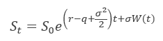
where r is the risk-free rate, q is dividend yield and W(t) is a Standard Brownian Motion under the risk-neutral probability Q.
As a refresher, we report the Black-Scholes time-t no-arbitrage price for a European call option:
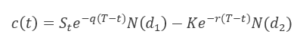
where N(z) is the cumulative distribution function of standard normal random variable, i.e.
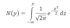
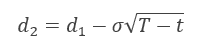
while
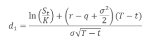
and
We do not report the formula for the European Put since it is similar to that of a European Call and can easily be derived using, for instance, the Put-Call Parity.
Now, if the option price is known (i.e. the option is traded), the Black-Scholes model can be used to calculate (through an iterative process) the volatility which is “implied” by the market.
Empirical evidence clearly shows that the implied volatility backed out from the premiums of liquid options is far from being constant. In particular, it shows different values for different Time to Maturity and Strike Price.
Firstly, let us focus on the Strike Price while keeping the Time to Maturity fixed. Options with different Strike Prices are associated with different level of implied volatility and a phenomenon known as Volatility Smile (e.g. for FX options) or Volatility Skew (e.g. for Equity options) can be observed.
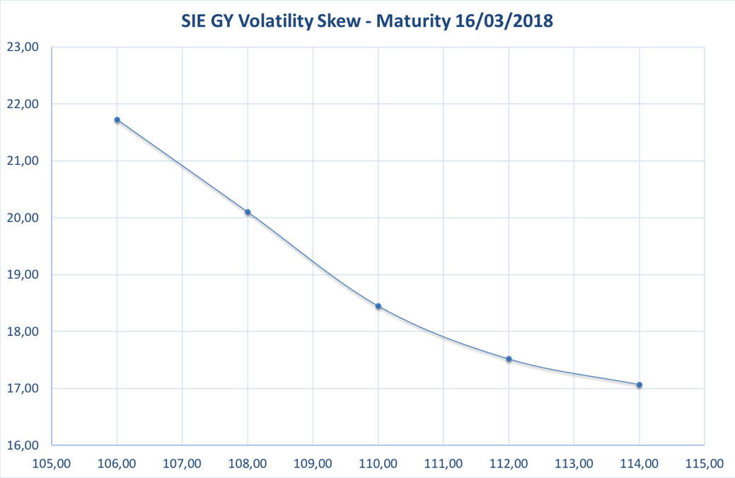
Chart 1: SIE GY Volatility Skew (source of chart data: Bloomberg, BSIC)
As an example, the graph above shows the Volatility Skew implied in the prices of the options on Siemens AG (ticker SIEGY) at different strike prices (reported on the horizontal axis).
Secondly, let us consider what happens when also Time to Maturity changes. Given that three variables are now being considered, a 3D plan becomes necessary for the analysis. Intuitively, what will emerge is a surface which basically is nothing more than several Volatility Skews combined together.

Chart 2: SIE GY Volatility Surface (source of chart data: Bloomberg, BSIC)
As an example, the graph above shows the Volatility Surface implied in the prices of the options on Siemens AG (ticker SIEGY) at different strike prices and at different maturities; five colours have been used to highlight various levels of Implied Volatility within the surface (see the legend at the bottom of the graph).
Given all these premises, it is now the right time to introduce the concept of Volatility Jump. Specifically, in reality, there are certain dates there is likely to be more volatility than average. These key dates are usually reporting dates (here the key dates are Earnings Announcements Dates, EAD). The implied volatility of an option whose expiry is after the date can be considered to be the sum of the normal diffusive volatility and the volatility due to the anticipated jump on the key date. In a nutshell:
TOTAL VOL = DIFFUSIVE VOL + JUMP VOL.
It theory, options of any expiry date after the key date could be used. In practice, the expiry date just after the key date is chosen. Trading an option whose expiry is just after the key date gives exposure not only to the implied jump, but also to the normal diffusive volatility. If the latter is not welcomed, a possible hedge could be a short position in the option just before the key date.
In order to calculate the implied jump, the normal diffusive volatility of the underlying needs to be estimated. Given that there are several ways to estimate the historical volatility, but only one implied volatility, the latter is to be preferred. Therefore, the option whose expiry is just before the key date is considered and its implied volatility is used as an estimate of the normal diffusive volatility. If such an option does not exist (maybe because the key date is extremely close to the current date) the forward volatility after the key date can be used as an alternative estimate.
The calculation of the forward volatility directly derives from the fact that variance is additive across time. Analytically:
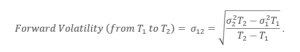
After having estimated the normal diffusive volatility and having computed the implied volatility after the key date, we are now ready to compute the implied jump. We start from:
![]()
from which we can get
![]()
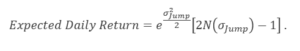
Finally, from the above implied volatility jump, it is possible to the implied equity return on the day of the jump, which is a combination of the normal daily move and the effect of the jump. Analytically:
Siemens AG: A Case Study for the Implied Jump
We now present the case study we developed to put the theory into practice. The stock chosen as the underlying of the options is Siemens AG (ticker SIEGY), that on 09/05/18 will announce its earnings related to Q2. As of 27/02/2018 (which is the date in which we downloaded the data from Bloomberg), the ATM option series with maturity 20/04/18 had implied volatility of 18.15%, while the ATM option series with maturity 18/05/18 had implied volatility of 19.15%. Using the formulae presented in the previous paragraph, both the volatility jump and the return jump were computed, resulting in values of 3.63% and 2.90% respectively. The same exercise was repeated for all the quarterly earnings announcements going all the way back to the beginning of 2009. A table summarizing our results is reported below.

Table 1: SIE GY Implied Jump Calculations (source of chart data: Bloomberg, BSIC)
In order to be as transparent as possible, we disclose that not all the earnings announcements were taken into account, the reason being that at some dates the implied jump and the implied daily return could not be computed due to fact the volatility term structure happened to be inverted. In theory, the volatility term structure before an earnings announcement should be upward sloping.
However, for all the announcements we took the data of the options exactly 71 days before the event in order to be consistent with our calculation for the 09/05/18 announcement. We believe that this wide period, between the announcement and the day in which implied jump and expected daily return were computed, could be the reason behind the inverted term structure in some of the dates. This is due to the fact that volatility moves with a stochastic mean-reverting process and usually after ca. 6-10 months goes back to its mean: hence, the more distant we are from a key date, the more mean reversion and stochasticity will play a role in determining the shape of the term structure.
Let us now look at Siemens from a more fundamental perspective.
Siemens AG (€87.53bn market cap, FY17 €83.049bn revenues, FY17 €6.179bn net income) is a Germany-based global industrial conglomerate, with operations spanning engineering, technology, energy and healthcare, offering its products and services to a diversified range of business customers across the world through 6 segments, 2 strategic units and its financial services arm.
The Power and Gas segment (18.6% of FY17 revenues, 10.3% net profit margin) produces gas turbines, steam turbines, generators to be applied to gas or steam power plants, compressor trains, and integrated power plant solutions, mainly used for generating electricity from fossil fuels and for producing and transporting oil and gas. Its main customers are public utilities and IPPs, companies in engineering, procurement and construction that serve utilities and IPPs, oil companies. The business is heavily exposed to national energy regulations (e.g. those on subsidies for renewable energy) and to the current shift from coal-fired to gas-fired plants, which is reducing demand for steam turbines. Due to these reasons, 2017 has been a tough year for the segment, which printed below expectation and below 2016 revenues and margins.
The Energy Management segment (14.8% of FY17 revenues, 7.6% net profit margin) provides software, products, systems and solutions for transmitting and managing electrical power and for creating distributed energy networks.
The Building Technologies segment (7.9% of FY17 revenues, 12.0% net profit margin) provides products, solutions, services and software for fire safety, security, building automation, heating, ventilation, air conditioning and energy management.
The Mobility segment (9.8% of FY17 revenues, 9.2% net profit margin) builds rail vehicles, rail automation systems, rail electrification systems, road traffic technology and provides related services especially to state-owned companies in the logistics and transportation sectors.
The Digital Factory segment (13.7% of FY17 revenues, 18.8% net profit margin) provides automation, data processing and other IT-related services to a diverse range of businesses.
The Process Industries and Drives segment (10.7% of FY17 revenues, 5.0% net profit margin) provides products, software, solutions and services for moving, measuring, controlling and optimizing all kinds of mass flows, e.g. gears, motors, converters, process instrumentation systems, process analytics devices, communication, industrial software.
The Healthineers strategic unit (16.6% of FY17 revenues, 18.1% net profit margin) provides medical technology, diagnostic imaging, laboratory diagnostics, software, clinical consulting services to the entire healthcare vertical.
The Siemens Gamesa Renewable Energy (SGRE) strategic unit (9.5% of FY17 revenues, 4.3% net profit margin) is a publicly listed company, created in April 2017 by the contribution of Siemens’ wind power business into the already existing Spanish publicly listed company Gamesa Corporación Tecnológica S. A. in exchange for newly issued shares: Siemens now holds the 59% majority stake. SGRE focuses on the development, construction, sale, operation and maintenance of onshore and offshore wind farms, having as main customers large utilities and IPPs.
The Financial Services (SFS) (19.9% after-tax ROE in FY17) segment supports Siemens’ customers’ investments with leasing solutions and equipment, project and structured financing in the form of debt and equity investments.
Below you can see the regional revenue split.
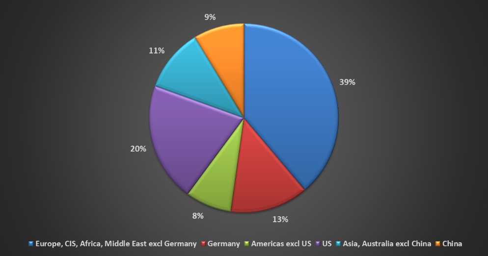
Chart 3: SIE GY Revenue Split by Region (source of chart data: Bloomberg, BSIC)
We will not try to forecast the precise EPS print of Q2 2018. However, in order to gauge the amount of uncertainty currently priced in Siemens options, we will look at four main drivers.
Firstly, in September 2017 Siemens and the French Alstom S.A. signed a memorandum of understanding to combine Siemens’ mobility business including the rail traction drives business, which is included in the Process Industries and Drives Division, with the publicly listed company Alstom. According to the memorandum, Siemens will receive newly issued shares in the combined company representing 50% of Alstom’s share capital assuming full dilution through exercise of all potentially dilutive securities and share-based payment plans. Further, Siemens will receive warrants allowing it to acquire Alstom shares representing 2% of its share capital, which can be exercised during the earliest four years after closing of the transaction. However, uncertainty remains. The transaction will be subject to Alstom’s shareholders’ approval, anticipated in the second quarter of calendar 2018. The transaction is also subject to clearance from antitrust and regulatory authorities. Closing of the transaction is expected at the end of calendar 2018.
Secondly, during FY17, Siemens announced that it intends to spin off and publicly list a minority stake in the Healthineers business in the first half of calendar 2018, depending on market conditions. This adds to pricing uncertainty.
Thirdly, uncertainty remains regarding the renewable energy space. In fact, after a volatile 2017 in Germany due to the reform of wind power subsidies (change of subsidies to an auction-based system) and a moving regulatory and tax-incentive environment in the US, the newly formed Siemens Gamesa Renewable Energy will need to cope with a possible turn in the Germany renewable framework and also in the UK one, especially under scrutiny given the possible changes due to the wider Brexit negotiations.
Finally, the recent tax overhaul in the US is expected to be EPS accretive to Siemens. However, Siemens’ guidance for a 27%-33% effective tax rate for 2018 is quite wide and we think that any change in the realized effective tax rate could materially impact any prevailing consensus on EPS.
Given the four above mentioned uncertainty drivers and the fact that our estimated implied return jump for Q2 2018 quarterly release (2.9%) is currently well below the historical average (3.23%), we would like to enter a long jump trade.
In order to accomplish this, we need to buy vol after the EAD and sell vol before the EAD, in order to be exposed only to the jump component: essentially, we are going long forward vol.
Therefore, we will go long an ATM straddle with expiry 18/05/2018 and current IVol of 19.15% (average put-call) and we will sell an ATM straddle with expiry 20/04/2018 and IVol of 18.15%. We will keep the position delta-neutral by buying or selling the adequate quantity of cash underlying. In this way, we will have pure volatility exposure. Furthermore, we will not be exposed to general parallel movements in the term structure: for a parallel increase in the term structure, we will gain on the longer dated straddle and lose on the shorter dated one (we need to weight the position to have equal initial vega across the two legs). The opposite is true for a down parallel move in the term structure. We are also hedged against reasonable moves in the skew as the legs are all ATM. We are only taking on the risk of a flattening of the term structure, i.e. of a downward repricing of the jump event.
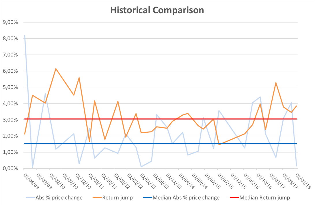
The main risk to this trade is that historically the implied jump has been higher than the realized absolute % price change. This can be seen by looking at the last column of Table 1 (“Deviation”). Here, we computed, from the beginning of 2009 up to now, the difference between the expected daily return (“Return Jump” in the table) and the realized absolute percentage price change on the day on the earnings announcement (“Abs % price change” in the table”). The summary statistics at bottom of the table point out that the mean and the median of the Deviation were 1.13% and 1.06% respectively. In a nutshell, we can say that the option market for SIE GY on average overestimates the actual percentage price change on the earnings announcement date. The graph below provides a graphical summary of this fact.


0 Comments