Systematic Credit Trading using Recurrent Neural Networks

Download PDF

Introduction

In this article, we determine whether recurrent neural networks can unlock any meaningful predictive power from a given feature set in forecasting corporate bond returns – or if the data is too noisy to yield reliable predictions. We explore whether these forecasts can be leveraged into building a profitable systematic credit trading strategy by building an out-of-sample back tester from 2013 to 2023. We take a different approach to the previous research done by the Bocconi Students Investment Club [1], by focusing solely on increasing the models’ predictive accuracy, rather than interpretability. Our first aim is to provide the reader with an intuitive explanation of what a recurrent neural network model is, before explaining how it is trained on our dataset to make predictions. We then construct two trade strategies to make systematic investments using these predictions.

The code for the article can be found on GitHub, at this link.

What is a Recurrent Neural Network?

Before diving into the trade strategy or the recurrent neural network model, we provide a simple explanation of a traditional neural network model, by making a comparison with the linear regression model.

A traditional neural network (NN) learns to map input data (such as numbers, words, or images) to output predictions (such as class labels or continuous values). This is similar to a linear regression model in that the goal is to find a relationship between independent and dependent variables. However, a linear regression model assumes a linear relationship between these variables, while a neural network can learn non-linear relationships.

For example, if we wanted to predict the price of a house based on features such as size and location, a linear regression might not capture their complex relationships, whereas a neural network model is able to learn the non-linear relationships and provide more accurate predictions in such a case.

There are similarities, and also differences, in the algorithms used to train linear regression models and neural network models. The aim of the training process in both models is to assign parameter values to the models in order to minimise a loss function (usually the mean squared error of the predicted and actual values). In a linear regression model, the algorithm minimizes the error between the predicted and actual output using Ordinary Least Squares (OLS) estimation. For neural networks, we use backpropagation [2], which is an algorithm that computes the gradient of the error and updates the model’s parameters to reduce this error. This is a more general method, capable of handling non-linear relationships.

In our back test, we use a more sophisticated version of the neural network model, namely the recurrent neural network (RNN) model. An RNN is a particular type of neural network designed for sequence prediction. It is particularly effective when the data has a temporal or sequential component, like time-series data or natural language.

The key difference, with respect to the standard NN, is that RNNs have memory. As opposed to learning the relationship between a single input and output for a given observation, they learn the relationship between several consecutive inputs and the output – an RNN processes data sequentially. This sequential nature is important for tasks such as generating text [3] or predicting bond returns, where past information of one variable (say variable A), can predict either future values of itself (variable A) or of another variable (say variable B).

The diagram below represents a simple RNN cell. At each time step t, the cell takes in two inputs: the current input x_t (e.g., a word in a sentence) and the hidden state from the previous step h_t-1, which carries information from past inputs. Inside the cell, these inputs are processed using a tanh activation function, which helps capture non-linear relationships. The output of this transformation produces the new hidden state h_t, which is then passed to the next time step. Additionally, an output O_t can be generated, depending on the specific task (e.g., predicting the next word in a sequence).

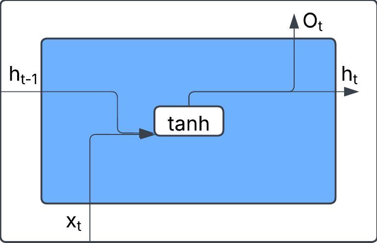
Figure 1, Source: BSIC

The formula for the hidden state in a simple RNN is:

The RNN cell above can be intuitively understood through a simple analogy: predicting the next word in a sentence. This analogy helps explain how the network learns from data and makes predictions. Imagine we trained an RNN model on millions of sentences from a variety of data sources. Specifically, we would use the first 5 words in the sentence as inputs and the final word in the sentence as an output. We then ask the model to predict the final word of an unseen sentence:

Input Sequence: “bananas are yellow, apples are …”

An RNN processes this sequence one word at a time, storing the context of what was said previously. It remembers that “bananas are yellow apples are”. Then, based on the sentences it has been trained on, it will predict the final word in the sentence. That is, it may predict that apples are “red” or “green” if it has learnt this information during training.

Note. In our back tester, we use Gated Recurrent Unit (GRU) Model – an improved version of the RNN that helps retain important information from sequential data. The main advantage of GRU is that it reduces the effect of the vanishing gradient problem, which occurs in standard RNNs when distant past information gets “forgotten.” GRUs use special gates (reset and update gates) that automatically decide which information to keep and which to discard. This makes GRU more efficient and faster to train than regular RNNs, while still capturing long-term dependencies.

Data

We further understand how the model works by explaining it in the context of our dataset. When we train an RNN model for predicting bond returns, we would use the past information of some variables (features) to predict the future values of another variable (bond returns).

Our panel dataset contains rows of monthly bond returns at time, t+1, and 8 features at time, t, for several bonds (~5000), for every month from 2002 to 2022. We chose the 8 features of the bond/company, which we believed may provide predictive power of the subsequent month’s bond returns. This was based on our own understanding of credit markets and research from [4]. The 8 features we selected were bond yield, credit rating, equity return, capital ratio, debt/EBITDA, debt/equity, interest coverage ratio and cash ratio.

If we were training our model with a traditional NN, it would simply learn the relationship between the 8 features at time, t and the bond return at time, t+1. However, as we are training an RNN it learns the relationship among the N (we choose N=5) previous sets of features and the bond return at time, t+1, capturing the temporal dependencies across those multiple time steps rather than relying solely on the features at a single time point.

Figure 2, Source: BSIC

Strategy Overview

For each month in our test set (2013 – 2023) we would use an RNN model to predict the subsequent month’s bond return for every bond in our investable universe. We would then construct our portfolio of bonds at the start of month, , to have long exposure to the bonds which the model predicts to have the greatest return, and short exposure to the bonds, which the model predicts to have the poorest return, through the month, t + 1. It is not as straightforward as training a single model on the entire 2002 – 2023 dataset and then using it to predict all the monthly returns, because doing so would introduce a look-ahead bias into our back test. Instead, we ensured that any prediction is made using a model trained only on data from before the test period. Therefore, we adopted an expanding window approach to train our models, on which we explain in the next paragraph.

We began by training our initial RNN model on data from 2002 to 2012, then use it to predict the returns for every bond (~3000), for every month, in the year 2013 to 2014 (roughly 36000 predictions). Once these predictions had been made and stored in the “results_list” dataset, we would then retrain the RNN model using the data from 2002 to 2014, and then predict the returns in the year 2014 to 20145. We repeated this process to obtain predictions for every year from 2013 and 2022. Therefore, in total, our back test trained 10 separate RNN models and generated around 360,000 predictions. We have developed a dashboard on the GitHub link to view the bond return predictions for each month in the test set. With this expanding window approach, our predictions can be considered out-of-sample. It is worth noting that we did not use cross-validation to optimise the RNN hyperparameters (layers, neurons, epochs). Instead we kept them consistent for each model. We then used these predictions to construct a trading strategy, exploring two different approaches:

1. Long Only Strategy – long the bonds which the model predicted to have the greatest returns throughout the following month.
2. Long/Short (L/S) Strategy – long the top predicted bonds and short the bottom predicted bonds.

We chose x = y = 3in our back test and the results in the next section are based on this. We factored in both transaction costs for trading the bonds and repo costs for shorting. Each month, our model identified different bonds to be long or short, and whenever one bond was replaced with another, we applied a 40bps transaction cost to account for the bid/ask spread. Additionally, for the L/S strategy, we applied a 20bps (annualised) repo rate for shorting the bonds. These cost assumptions are based on investment-grade averages. A further step we could have taken would be to optimize the hyperparameters and to maximize overall returns (or Sharpe ratio). However, this would have required a proper cross-validation approach to avoid introducing a bias into our model. It would not have been valid to simply test various and combinations, pick the one that maximises returns, and still claim unbiased results. However, we do look at how the strategy performs for different combinations later on as a robustness check.

Results

Below, we display the strategy using absolute bond returns (left) and bond returns with interest-rate risk hedged (right), both after transaction costs. Considering the absolute bond returns, the Long only strategy considerably outperformed the benchmark achieving a 2.07 Sharpe ratio across the total period and 12.5% annualized returns. The L/S strategy exhibited a poorer performance, obtaining an overall Sharpe ratio of 1.29 and underperforming the benchmark. With interest-rate risk hedged returns, the Long Only strategy performed well across the test period, obtaining an overall Sharpe ratio of 1.52, outperforming the benchmark. The L/S strategy had a poorer performance, obtaining an overall Sharpe ratio of 0.96 and underperforming the benchmark.

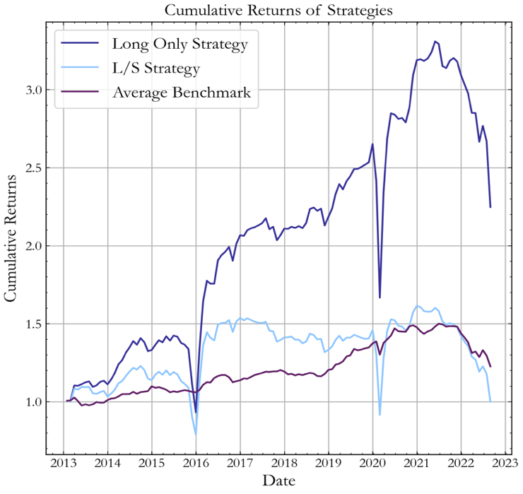
Figure 3, Source: BSIC

For the remainder of the article we will dive deeper into the results of the interest-rate risk hedged portfolio. We are more interested in these results as the profits in this portfolio were solely driven by changes in credit spreads (rather than interest rates). The L/S strategy underperformed, largely because of high transaction and repo costs. As, on average, the L/S strategy traded twice as many bonds as the Long only strategy, the number of transactions, and therefore costs, were doubled. In addition, paying a repo rate to short the bonds reduced overall profitability. On the other hand, the Long Only strategy performed well throughout most of the period, except in 2015 and early 2020, where it experienced drawdowns. The distribution of monthly returns are displayed below:

Figure 4, Source: BSIC

We evaluate the model’s performance by comparing its bond return predictions to actual outcomes. In Figure 6, we compare the model’s predicted bond returns for July 2018 with the actual bond returns observed over that month (the month was chosen arbitrarily to provide an example). The model’s predictive accuracy, as measured by MSE, was weak, indicating its inability to accurately forecast the bond returns – a result which was expected due to the stochastic nature of bond returns. Nonetheless, in the majority of cases, the bonds which the model identified as having the highest returns did indeed exhibit positive returns, meaning that on average the Long Only strategy carried a positive expected return.

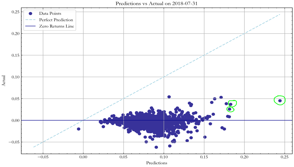
Figure 5, Source: BSIC

In other words, by looking at the top 3 bonds the model selected based on the predictions above, we can see that the true average returns were positive. Although, there was a large mean squared error in the predictions, the strategy still chose bonds leading to an average return of 4.0% throughout July 2018.

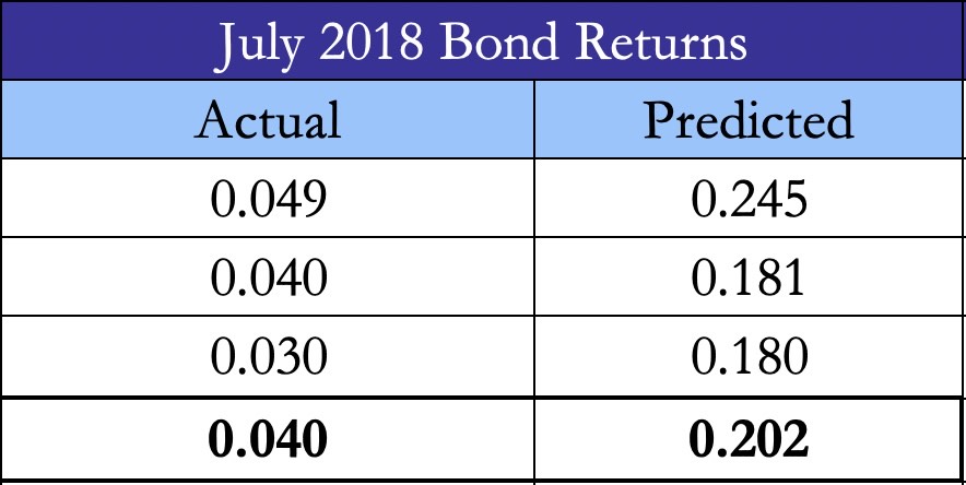
Figure 6, Source: BSIC

Referring back to Figure 3, the strategy performed particularly well in 2016 and throughout the second half of 2020 as the model was able to detect bonds which would yield significantly high returns. However, as stated previously, in 2015 and Q1 2020, the strategy underperformed the benchmark by selecting bonds that ultimately performed poorly. In general, when corporate bond markets were bullish, our portfolio outperformed significantly, but underperformed in bearish market conditions. Summary statistics of both strategies are displayed below:

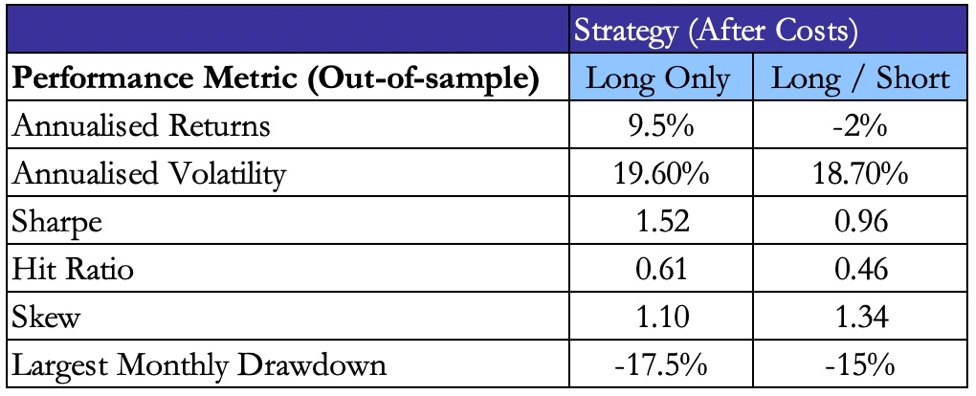
Figure 7, Source: BSIC

Robustness Checks

When running a back test it is important to understand how sensitive the model’s performance is to changes in hyperparameters.

We simulated ex-post returns for different values of N, where N is the number of top (bottom) performing bonds we long (short) in our back test. While the results of this robustness check should not be used to pick the optimal N ex-ante when calibrating the model, they represent a way to gain knowledge of what would have happened if we had chosen a different N when formulating the strategy logic. In order to make performance figures more interpretable, we compute strategy returns as net of transaction costs.

The figure below shows back tests of the model’s performance for N = 1, … ,10. Although the evidence shows that performance changes significantly for different N, we observe decreases in performance as N increases. The explanation for this is the trade-off between diversification and the transaction costs of higher N. The monthly rebalancing of a Long only portfolio of N bonds can involve replacing up to N bonds with new ones. For what concerns the L/S portfolio, it can involve replacing up to 2Nbonds.

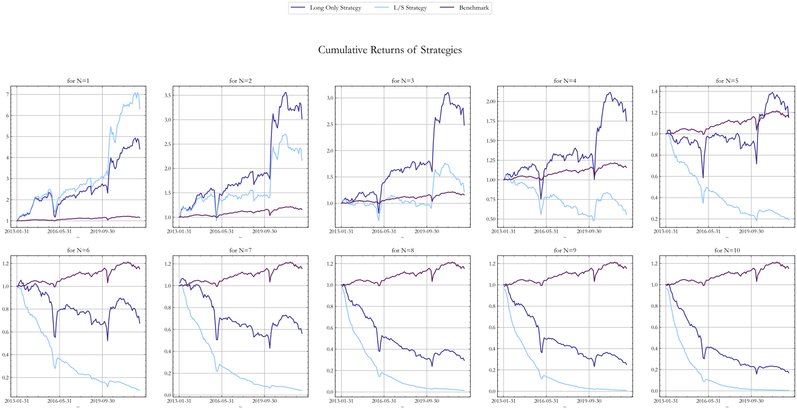
Figure 8, Source: BSIC

Factor Analysis

To gain further insight, we also performed a factor analysis of the strategy against the main factors driving credit returns: value, duration, equity momentum and bond age [5]. We ran a regression of the monthly bond returns against the returns of these factors and the regression results are displayed below:

Figure 9, Source: BSIC

Throughout the period only the Value and Equity Momentum factors were statistically significant and explain most of the variance. Although on average the strategy was long equity momentum and short value, these exposures changed significantly throughout the period, highlighting the model’s ability to harvest risk premia.

Figure 10, Source: BSIC

Conclusion

In conclusion, our results showed that during the test period, RNNs were able to predict the bond returns with enough accuracy to generate a profitable trading strategy. The Long Only strategy outperformed the L/S strategy and the benchmark both in terms of cumulative returns and Sharpe ratio due to positive expected returns, a small set of high performing bonds, and minimal transaction costs. Possible avenues for further research include 1) Extending the RNN model to include an attention mechanism, improving interpretability. 2) Developing a more comprehensive feature set, based on further literature and undertaking a robust feature analysis. 3) More accurately modelling transaction and repo costs by taking industry, rating and liquidity into account, rather than applying a fixed rate to all bonds.

References:

[1] “A Systematic Approach to Credit Investing”, Markets Division, Bocconi Students Investment Club, 2024

[2] “A Gentle Tutorial of Recurrent Neural Network with Error Backpropagation”, Chen G.

[3] “Deep Learning”, MIT Press, Goodfellow I. J. and Bengio Y. and Courville A., 2016.

[4] “Common factors in corporate bond returns”, AQR Capital Management, Israel R., Palhares D., and Richardson S, 2017

[5] “Corporate Bond Factors: Replication Failures and a New Framework”, Dick-Nielson J., Feldhütter P, Pedersen L. H., and Stolborg C.