An Introduction to HFT
High-frequency traders (HFTs) account for a large proportion of the trading volume in security markets today. Despite this, there is very little understanding of the overall industry. We believe that you, the reader, should be made aware of this little-known yet massively impactful industry and all of its fascinating nuances. As such, throughout the article, we explore the basics of market making as well as a brief history of how HFT systems behind it have evolved through time. On the more technical side, we explain, on a high-level, the process of determining fair-value and inventory management, the world of infrastructure and networking in the context of HFT, as well as a simple application of Avelleneda-Stoikov, a staple model in the world of HFT.
Dealers
The role of a market maker in securities markets is to provide liquidity on the exchange by quoting bid and ask prices at which he is willing to buy and sell a specific quantity of assets. In recent years, with the growth of electronic exchanges, anyone willing to submit limit orders in the system can effectively play the role of a dealer. Specifically, HFTs are firms that perform this function using advanced infrastructure to do this job as efficiently as possible. That’s their business model as wholesalers: using technology to efficiently commit capital and bridge the gap in time between when buyers want to buy and sellers want to sell.
Contrary to the common perception that HFTs have some unfair advantage, unfair access to exchanges, and the ability to manipulate or move markets in ways regular trading firms cannot, their real advantage lies in technology. For example, the servers owned by HFT shops are located on the same sites as the exchanges’ computers and this allows them to get prices split seconds before the public, because of discrepancies in connection speeds.
From the exchange’s perspective, HFTs technically have the same access as everyone else. However, this “equal access” comes at a very high price, effectively limiting it to firms that can afford the infrastructure and connectivity costs.
Evolution of the Industry
The days of Flash Boys have passed, and HFT has entered a new era. After its development in the mid-2000s, HFT entered a phase of explosive growth, leading to the rapid rise of small trading shops but also to the dominance of today’s large and highly profitable firms. As more players entered the space, including fintech firms, competition intensified and eventually gave way to consolidation. Now, the major players are well-known market makers such as Citadel Securities and Jump Trading.
HFT strategies have also been broadened out of equities to more asset classes including FX, ETFs, and cryptocurrencies. If the firm focuses on a relatively new asset class, there is also a component of “dirty work” that is super important such as understanding the APIs, normalization of data, seeing what’s missing in the documentation, and measuring latencies. In this space, firms can either go make markets on a well-established exchange and focus on alpha generation or pick some long-tail exchange and try to figure out the infrastructure specifics around that exchange.
In traditional markets this matters less because the systems are more standardized and robust. But in asset classes such as crypto, every exchange has its own quirks and the better you understand the infrastructure, the more likely you are to find edge.
These firms are also aiming to work smarter, not only searching for speed. Physical limits are starting to show, and there’s only so much more time that can be shaved off. They were in the realm of saving nanoseconds and the technology to save such time is about to get more and more expensive. It’s reaching a point where firms need to invest in significant amounts to stay ahead from a latency perspective.
As a result, firms are moving beyond pure speed and focusing more on signal generation, performing backtests and building strategies that are not only faster but also smarter. This is seen as the blend between HFT and ‘mid-frequency-trading’, which is a concept that goes beyond the scope of this article but is nonetheless a very important, novel element to modern-day HFT firms. Without further ado, let’s dig into the more technical aspects of this ‘hidden’ industry and define some simple concepts before moving forward.
What is a Limit Order Book
When talking about how HFT operates, a term which is often mentioned is LOB (Limit Order Book). A book is basically a collection of bid and ask orders, each with its own price and size. The bottom of this book consists of bids while the top comprises the asks. This is pretty obvious since the bids are ranked such that higher prices gets priority while the opposite happens for asks. In this way the best ask and the best bid are the first to be served when a transaction occurs. The spread between these two quotes is often called the bid-ask spread. A common approach amongst exchanges is to use something known as a central-limit order book (CLOB) where the timing of the quote determines first priority while sizing is the penultimate priority.
Market Making
When speaking about market makers, it’s very important to note that they operate in a distinct way to other market participants. At its core, a market maker doesn’t care about taking a directional view on the asset, what matters is getting filled on both sides. As long as two-sided flow exists, that is, they get filled often enough on both the bid and ask side without market participants determining and re-pricing a new ‘fair-value’ over a large number of trades, they will profit simply from collecting the spread. Now, we will expand on some of the main components that are involved in market making:
Fair value
Before a market maker decides an optimal price to quote their bids and asks at, they must first form a belief of where the asset should be trading. As such, fair value becomes of paramount interest, which is the price around which the market maker quotes. This value often originates as the mid-price (the average of the lowest ask and highest bid) on one exchange or aggregated across many if the asset trades upon multiple values (taking into account of the volume on each exchange, of course!). However, since market makers seek edge in determining ‘fair’, they often incorporate other signals which may help the market maker to mitigate the prospect of getting picked off from other informed participants and improve their edge.
One may wonder, “Okay, so what does this mean in practice?” Well, a simple way to think about is as follows: imagine a market in which all the participants are uninformed, meaning when a buy or sell order happens, it is uncorrelated with the direction in which the market moves, then if a market maker simply quotes around the current price, over a large number of trades it will make a profit in expectation from the spread they charge. This is what market makers like to call ‘uninformed flow’.
Real markets, however, also contain informed flow. In that case, simply quoting around the current price is not enough; a market maker that is faster and can see the mid-price has changed can take advantage of your stale quotes or someone that has a better forecast of the future price can trade against your orders when they are mispriced. When this happens, you’re on the wrong side of adverse selection: you’re more likely to be filled when your quote is bad, and you end up trading against what’s often called toxic flow.
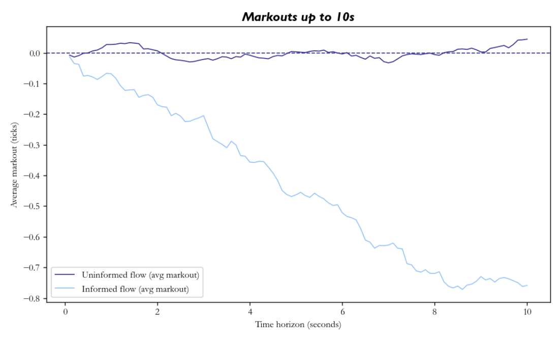
A simple check which market makers use to detect adverse selection is the use of markouts; for each fill, they look at how much the mid-price changes after a fixed horizon (say 1 second or 5 seconds) to see whether, on average, the market moves for or against them after they trade.
In the chart below, we plot average markouts as a function of time after we get filled, we can perfectly see the effects of adverse selection. We ran a simplified model where the mid follows a random walk, and we quote a fixed spread around the mid, with market orders arriving according to two independent Poisson processes: one uninformed (with random buy/sells), and one informed where traders have a probability  of predicting the direction of the mid-price at a future horizon.
In the uninformed case, the markouts stay close to zero, whereas in the latter case of informed flow, we can see that markouts start near zero but drift negative as we move out in time, as those informed bets realise.
So, naturally, we can see why a market maker should incorporate some sort of forecast in its fair value; to protect itself from adverse selection and to improve its edge. One example of a signal, albeit slightly outdated, is orderbook pressure, which is essentially a size-weighted average of the best bid and the best ask:

Another basic signal is order book imbalance, which is going to take a value between -1 and 1, and measures how unbalanced the volume on the bid and ask side in the top N levels:

where  is the volume in the top N levels on the bid side (ask side).
Both signals make sense as valid predictors when one considers how market orders will affect the mid-price. Suppose the imbalance is strongly positive, so there is more liquidity on the bid side. Then when a buy market order arrives, it hits the thinner side of the book and is more likely to completely consume the best ask, thus moving the mid-price up. In contrast, when a sell order arrives, it needs more size to deplete the liquidity at the best bid. If orders arrive randomly then the thin side of the book has a higher probability of getting depleted first, therefore the future expected price should be skewed in that direction.
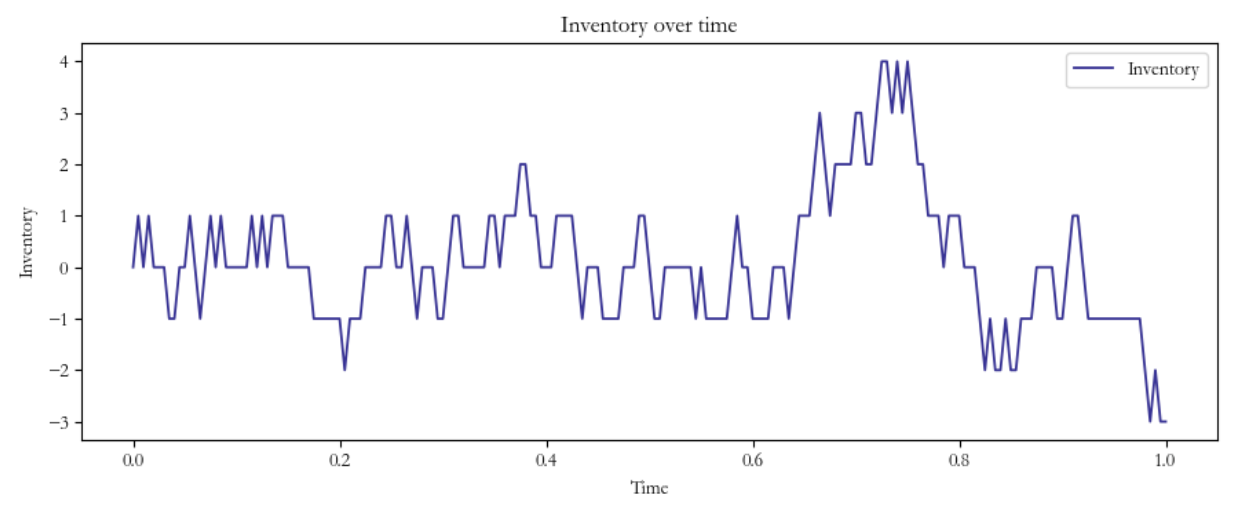
Inventory Management
As a market maker, you are frequently buying and selling on the market. By doing this it’s natural to have a positive or negative inventory since it’s highly unlikely to make symmetric, simultaneous trades. If this were the case, market-making would be trivial! However, evidently, this is not the case. This ‘inventory’ of the traded asset can therefore constitute a risk for an HFT firm, as they’re now subsequently exposed to directional risk, a generally unwanted feature. In this position, firms consider ‘skewing’ their quotes such that this inventory risk is offloaded.
In order to properly grasp this ‘skewing’ concept, let’s consider a simple scenario: as a market maker, your ask orders get hit by quite a sizeable amount. In other words, you are now short the quoted asset. What should you do? Well, you should skew your quotes; try to get crossed for your bid (in other words, buy the asset cheaper) by a proportionate amount to mitigate directional risk! This can be done by quoting tighter bid prices with large size around the perceived fair value while conversely quoting wider ask orders with smaller size. Naturally, what this does is increase your probability of offloading this unwanted inventory risk. Sure, you’re probably not going to make as much money compared to the perfect two-sided flow scenario, but you’re making sure that you’re protected against unwanted price swings in the underlying.
So now, you’ve become familiar with some basic market making concepts, but what’s actually happening underneath the hood? In other words, how does technology come into play here?
Networking
Latency is one of if not the most important element within HFT. Latency is the name of the game and can be the determining factor of whether you have edge in this industry or not. To understand why, take a simple making strategy: if one wished to consistently execute at the top of the book in a dynamic market, slower latency would prevent you from competing with flow from other, more fast competitors. Additionally, in the case of toxic flow, your ability to react is stifled, and your quotes may be picked off as stale liquidity when information dictates fair value price changes.
As you can see, it’s incredibly important to have speed, and while not every HFT firm is naturally employing such a strategy, it’s still quite evident that the principle to some extent will still hold. So, how exactly do HFT firms optimize this portion of their strategy? Well, it’s partially two elements: infrastructure and networking.
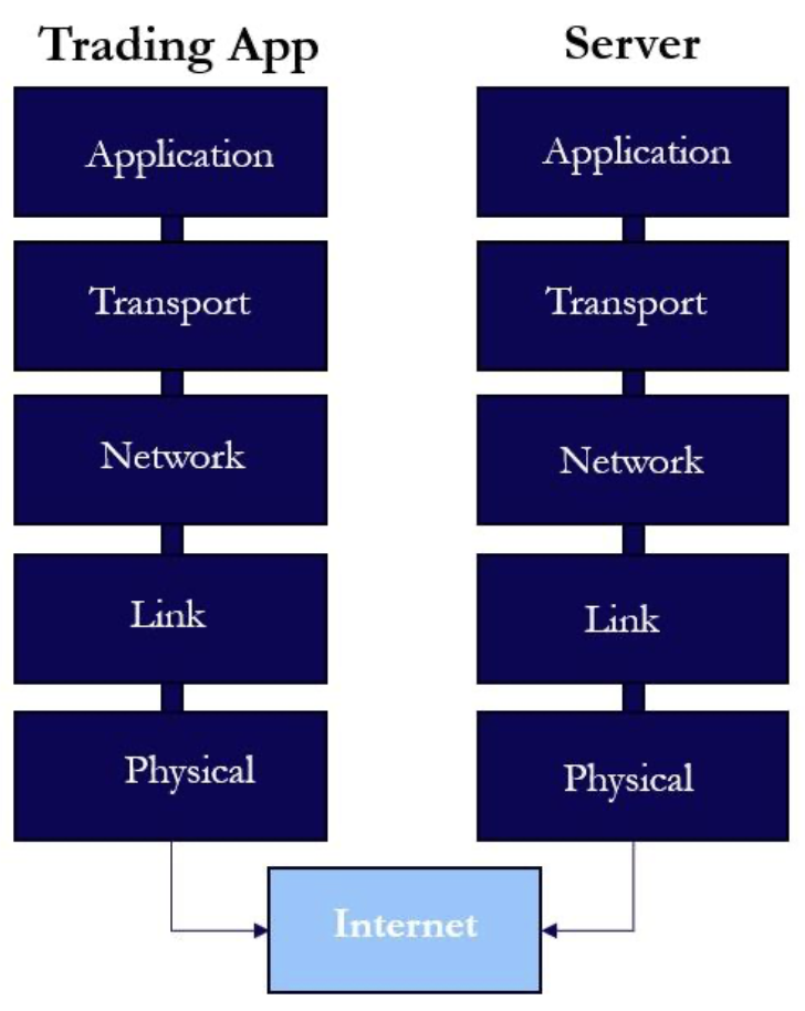
Networking refers to all the layers that move bits between the HFT’s process and the exchange; in other words, it’s the way in which our requests to quote or take trades with the exchange are actually executed. A high-level abstraction of networking can separate the concept into 5 distinct layers.
Layer 1: Physical – the actual, physical transmission of bits between parties
Layer 2: Data Link – transformation of bits into interpretable communication across network devices in the form of frames (i.e. Ethernet)
Layer 3: Network – handles data forwarding via IP addresses across different networks, distinct from L2 due to larger reach across multiple networks
Layer 4: Transport – moves data between applications using ports (i.e. TCP)
Layer 5: Application – the actual messages and semantics your software speaks (i.e. HTTP/TLS/FIX/ITCH)
Chronologically, each of these layers build on top of each other in order to provide the necessary protocols for network devices to interact with each other at a high level. For the sake of HFT, each of these layers is absolutely crucial for optimization, as each layer is additive in terms of latency contributions. A useful diagram to understand this interplay can be seen below:
So, how do they do it? Well, if we knew, we certainly wouldn’t tell you! Just kidding. Although the actual practices behind HFT doors are guarded with alleged 3-headed monsters, we can certainly deduce in broad strokes the ways in which these firms would go about optimization. And, for the sake of simplicity, we will solely focus upon layers 3 through 5 due to them being the most customizable from the firm’s perspective.
On the networking layer, the main answer is quite straightforward: host your server as close to the exchange server as possible. Furthermore, packet routing in the most effective manner to avoid unnecessary latency is a must. This generally comes in the form of choosing fastest physical routes which minimizes hops and jitter (variability in latency). From a hardware point of view, the firm should be striving towards using ultra-low-latency (ULL) switches.
Next, on the transport layer, exchanges usually use UDP for market streaming due to priorities of minimal latency over packet loss, whereas for order submission, TCP is used due to the reliability of the delivery. From the HFT perspective, TCP optimizations for order submission must be made: Nagle’s algorithm, a process which waits for certain critical messages to be aggregated before sending, is usually disabled to speed things up among other considerations to minimize stalls.
Lastly, for the application layer, binary protocols are chosen for messages, unnecessary headers and elements in the payload are removed, and finally, our trading infrastructure must be optimized.
Infrastructure
We are officially in the weeds. This is one of the most important and non-trivial problems that exists in HFT development, so we decided to write its own little subsection to sufficiently appreciate the nuances.
The first concern is choice of programming language. Generally, in HFT, there are two languages market makers consider in response to this concern: Rust or C++. Both being low-level languages with further customizability on lower levels of operations, they make for fine choices with their own sets of trade-offs.
For instance, one of Rust’s main advantages is its ability to prevent major memory issues at compiling times. This is essential when considering jitter minimization, as memory leaks and other problems manifest in latency variability. C++ gives you more freedom regarding memory which can be especially handy for a veteran, but for less adept users, this increased freedom may lead towards dreaded memory leaks.
With regards to the ecosystem, however, due to C++’s seniority and mass developer following, NIC stacks and exchange tooling is in abundance on the older programming language relative to Rust. In brief, Rust gives you certain guardrails for low-level language standards while C++ enables freedom with a more battle-tested ecosystem.
“What’s the point of doing all this stuff?”, you may be thinking. Sure, you can see that we want to optimize latency, but how do the aforementioned considerations help achieve this feat? Well, there’s 3 main concerns at this level: cache misses, memory usage, and threading. Firstly, cache misses occur when code frequently jumps around memory, meaning that the CPU must access slower levels of memory in order to perform its function. We naturally wish to minimize those instances, and that happens through memory usage/allocation. Specifically, we want to remove dynamic allocation, fragmentation, as well as the releasing of memory in order to decrease latency and jitter. Lastly, multi-threading, which refers to multiple processes running parallel to one another, is essential to HFT due to the sheer speed processes must be performing at. Unfortunately, running processes side-by-side naively may lead to context switches, locking contention, migration between cores and so on, all contributing to jitter and tail latency. As such, we need to design code which minimizes these locks and properly isolates “hot” threads which are of the utmost priority.
There’s a lot of words here, and some of them may be difficult to interpret, so a useful analogy here is to think of these elements as the components of a race car and each of these problems as a potential bottleneck for its speed. It needs to be the fastest, so although the car may work in the presence of them, it won’t win the race. When you’re optimizing infrastructure and networking at an HFT firm, you are essentially a financial mechanic, working with Rust/C++ and TCP optimization instead of grease and metal: not as sexy, but it pays pretty good!
Avellaneda-Stoikov model
Back in the days, market making was gut instinct and superstition, but in 2006, Avellaneda and Stoikov turned it into an optimization problem, laying down the first foundational framework. In the paper [1], the authors studied a market maker’s two main concerns: dealing with inventory risk and finding the optimal bid and ask spreads.
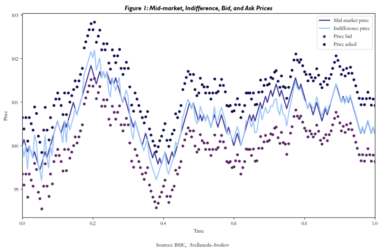
As we said, the basic strategy for market making is to create bid and ask orders around the market mid-price. Although we introduced some approaches to further sophisticate fair-value calculation, our quoting mechanism hasn’t yet accounted for inventory risk. The paper by Avellaneda & Stoikov aimed to address this risk by adequately skewing through a new reference price, (the reservation price) which is not simply the mid-price, but rather the market maker’s own ‘adjusted’ valuation of the asset, based on three main factors.

Where s is the stock price, q measures how far the market maker’s inventory is from the target level (usually zero),  is the value (defined by the market maker) which accounts for their tolerance level of inventory risk, and
  is the time until the trading session ends.
As the trading session is nearing the end, the reservation price will approach the market mid-price, reducing the risk of holding the inventory too far from the desired target.
The negative sign preceding the adjustment term helps us understand the logic. When the position is long, this term is negative, lowering the reservation price. This occurs because the agent seeks to reduce excess inventory and by decreasing the internal valuation of the asset, the market maker effectively signals a willingness to sell at a price below the current market mid-point, encouraging potential buyers. Conversely, when the position is short, the term becomes positive, and the aforementioned logic still applies.
Optimal spread
Once the reservation price is established, the optimal bid and ask quotes are derived:

Where  .
.
These quotes represent the prices at which the market maker is willing to transact.
As you can see above, a new factor k is introduced. This latter represents the order book “density”. There are many different models with varying methodologies on how to calculate this parameter. An elevated k value, indicates that the order book is denser, and the optimal spread will have to be smaller since there is more competition on the market. On the other hand, a smaller k assumes that the order book has low liquidity, and a more extensive spread would be more appropriate.
The execution logic of the model is now straightforward: we calculate the reservation price based on what is the target inventory, we derive the optimal bid and ask spread and we create market orders using the reservation price as reference.
 A few considerations on the model
These findings may seem promising upon the surface and adequately represent a simple representation of the “academic” framework, but a few considerations need to be made…
Firstly, the Avelleneda-Stoikov assumptions are, by nature, simplified. Stock prices are assumed to move by a geometric brownian motion with a fixed volatility term, not adequately reflecting the dynamic nature of volatility. Secondly, the filling of orders is assumed by random and independent jumps modelled via a naive poisson process, while in reality, they tend to cluster and influence each other.
Secondly, we blatantly ignore the fact that our trading may create a type of ‘ripple effect’ in terms of perceived market information and consequent price swings.
Next, there are also challenges in parameter calibration and limitations of market microstructure. In reality, the parameters in the model are not stable. Despite this, we still assume that risk tolerance is constant and uses a baseline curve to determine how the probability of a fill decreases with distance.
In terms of microstructure, markets have minimum price intervals, and orders are executed sequentially at each price: the continuous model ignores these factors, ignoring important aspects that determine the probability and speed of execution.
References
[1] Avellaneda, Marco; Stoikov, Sasha. “High-Frequency Trading in a Limit Order Book”, 2006.
[2] Quant arb, “Advanced Market Making”, 2025


0 Comments