Trading Credit Derivatives

Introduction

In this article, we introduce the main market-traded credit derivatives, with a particular focus on Credit Default Swaps (CDS). After explaining how they work, we delve into the terminology and pricing mechanisms, covering single-name CDS, indices such as iTraxx and CDX, and CDS options. Next, we explore relative value strategies in the credit space: from basis trading to macro views based on IG vs HY, to arbitrage between an index and its components. We also provide an overview of the CDS index options market, a tool that has become increasingly popular for gaining targeted and leveraged exposure to credit risk and volatility. Finally, we conclude with a backtest of a credit spread arbitrage strategy, applying a pairs trading approach to the credit space by trading the mean reversion between the OAS spreads of two ETFs.

From Bond to CDS

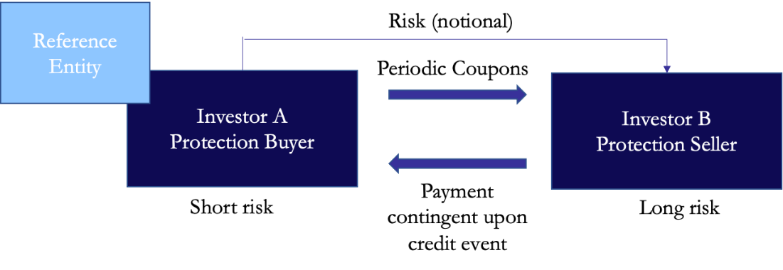
A credit derivative is a financial contract that allows one to take or reduce credit exposure, generally on bonds or loans of a sovereign or corporate entity. In a credit default swap (CDS), one party purchases credit protection from the other to cover the loss of face value of an asset following a credit event, where the protection buyer is short risk. Protection lasts until a maturity date and until then, the protection buyer makes quarterly payments to the seller, called the premium leg. These payment amounts are determined by the spread of the CDS, adjusted for frequency. The other leg of the swap is the protection leg – if a credit event occurs & payment is made by seller to buyer, in which case payment is the difference between par and the price of assets of reference entity on face value of protection. CDS indices are tradable products that allow investors to establish long or short credit risk positions in specific credit markets or market segments.

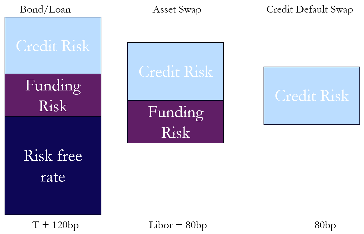
The diagram below illustrates how the total yield on a corporate bond can be broken down into its components (risk-free rate, funding risk, and credit risk) and how these relate to asset swaps and CDS pricing.

CDS Single Name Pricing

The price of a CDS directly reflects the implied probability of default of the reference entity. Factors affecting this price are credit rating, market sentiment, liquidity and economic conditions. Resulting pricing formulas depend on the choice of underlying models used to describe different dynamics such as default event, interest rate or the loss given default. In any case, the price is determined by the comparison between the present value of the expected premium payments (what protection buyer pays) with the present value of the expected protection payments (what protection seller pays in case of default). There are some model independent formulas given the initial zero-coupon curve observed in the market and the survival probabilities, for example: the CDS price at a time t=0 is given by:

$CDS_{ab}(0, R, LGD;~\mathbb{Q}(\tau > \cdot)) = \text{Prem } L_{ab}(\mathbb{Q}(\tau > \cdot)) - \text{Prot } L_{ab}(\mathbb{Q}(\tau > \cdot)) = R \left[ -\int_{T_a}^{T_b} P(0, t)(t - T_{\beta(u)-1})\, d\mathbb{Q}(\tau \geq t) + \sum_{i=a+1}^{b} P(0, T_i) \alpha_i\, \mathbb{Q}(\tau \geq T_i) \right] + LGD \int_{T_a}^{T_b} P(0, t)\, d\mathbb{Q}(\tau \geq t)$

where: R is the CDS spread, P(0, t) is the discount factor, α_i is the accrual fraction for each period, and $\mathbb{Q}(\tau \geq t)$ is the survival probability up to time t.

The buyer usually pays a periodic fee and profits if the reference entity has a credit event, or if the credit worsens while the swap is outstanding. When a credit event occurs, the contract is triggered, and the seller must pay the buyer. This can be facilitated either through physical settlement (where the buyer delivers a bond from the defaulted entity and seller pays face value in return) or through cash settlement. Credit events stretch beyond bankruptcy, to defaulting for reasons other than bankruptcy, failing to pay outstanding debt obligations/obligation acceleration (obligations are moved & issuer must pay debts earlier than anticipated), or a restructuring of a bond or loan. For a corporate CDS, the most common triggers are failure to pay, bankruptcy and sometimes restructuring, whereas for sovereign CDS, the causes are mostly failure to pay and repudiation/moratorium. The latter occurs when there is a dispute in the contract validity and the contract is suspended until those issues are resolved.

The structure of a CDS can be seen in the diagram below: the coupon payments made from buyer to seller on an annualized basis are calculated by multiplying the notional amount of the swap, by the market price of the credit default swap. CDS market prices are quoted in basis points (bp) paid annually.

Index Pricing

CDS indices reflect the performance of a basket of single-name credit default swaps (CDS on individual credits). Unlike a perpetual index like S&P 500, CDS indices have a fixed composition and fixed maturities with equal weight given to each underlying credit in the index. A new series of indices is established approximately every 6 months with a new underlying portfolio and maturity date, to reflect changes in the credit market and to give the indices a consistent duration of approximately 5 years. If there is a credit event in an underlying CDS, the credit is removed from the index.

Each index is a separate, standard CDS contract with a fixed portfolio of credits and a fixed annual coupon. Investors will pay or receive a quarterly payment of this fixed coupon on a desired notional. The benchmark indices for Europe are the iTraxx Main Index and the iTraxx Crossover Index. The former is constituted by the 125 most liquid investment-grade European corporate CDS names across different sectors, while the latter includes the 75 most liquid high-yield (rated below BBB) corporate CDS names. Both are rerolled every March and September, each being assigned a new Series number and rebalanced monthly.

When a new index is launched (on the run), off the run indices (now outdated) continue to trade until maturity and investors are not obligated to move their positions from off the run to on the run, although on the run will be more liquid and most funds will roll over with the rebalance. On the run indices are more liquid and more closely reflect market sentiment, with a wider availability of quotes. Indices moves quicker than underlying credits as investors can express positive/negative views about the broader credit market in a single trade with the index so there is greater liquidity. On the run indices trade at a wider spread as investors wanting to short credit use this as it is more liquid, whereas off the run indices are more frequently used by long risk investors who like to hold the index for longer and benefit from the roll down effect.
The price of an index is expressed as a CDS spread in bps per year. The fair spread is calculated using the current market spreads of each constituent single name CDS.

Basis

The first trade we want to introduce is the basis trade. The bond-CDS basis is the difference between the full running CDS spread and a bond spread measure- usually the Z-spread (a constant spread added to the risk-free yield curve to match the bond’s price), the asset swap spread, or the par equivalent CDS spread. The rationale behind this strategy is that, in theory, a bond combined with CDS protection should replicate a risk-free asset. By hedging the credit risk, the investor is exposed solely to the relative pricing between the bond and the CDS. Under ideal market conditions, the bond spread should match the CDS spread, and any deviation creates a potential arbitrage opportunity.

If the basis is negative, then the CDS spread is lower than the bond spread. To capture the pricing discrepancy when a negative basis arises, an investor could buy the bond and buy CDS protection (short risk) with the same maturity as the bond. If the basis is positive, then the CDS spread is higher than the bond spread. An investor could borrow and short the bond and sell CDS protection (long risk) with the same maturity (or as near as possible) as the bond. Thus, the investor is not exposed to default risk but still receives a spread equal to the bond-CDS basis.

Negative basis trades are more attractive than positive basis trades. Indeed, in a positive basis trade, an investor needs to repo the bond and sell CDS protection. The difficulty with repo of corporate bonds and the cheapest-to-deliver option that protection buyers own makes positive basis packages more difficult to analyse and execute.

We highlight some of the most important drivers of the Bond-CDS basis. The direction of the basis will be a function of which of these drivers.

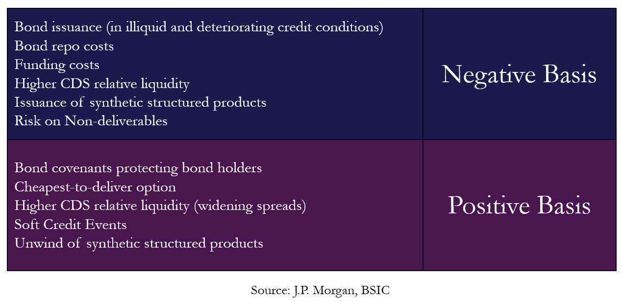
Considering the current European macro environment, the basis is being influenced by elevated funding costs (which make it less profitable to hold funded positions in bonds) and as a result, investors show a preference for the more liquid CDS market, which compresses derivatives spreads relative to bond spreads. In addition, more challenging conditions for bond issuance persist. In fact, companies issuing new bonds must offer higher spreads to attract capital, pushing the basis even lower. However, a negative basis does not automatically imply an opportunity for profitable arbitrage.

Negative basis trades become profitable only if the basis is negative enough to exceed the so-called “Breakeven Basis”, that is the level at which the annual income of the trade exactly covers the funding costs.

The main drivers of the Breakeven Basis are the unsecured and repo funding rates as well as the bond price as shown in the formula: $\textit{Basis}_{\textit{Breakeven}} = -\textit{F} - \textit{mF} + (1 - \textit{h})(\textit{F} - \textit{R}) \dfrac{\textit{P}}{100}$

Where $\textit{F}$ is the unsecured funding rate, $\textit{m}$ is the CDS margin, $\textit{R}$ is the repo rate, $\textit{h}$ is the repo haircut, and $\textit{P}$ is the Bond dirty price.

CDS-Stock

Another trade we can discuss exploits the inverse relationship between a company’s CDS spreads and its equity price. These are linked through credit risk – when credit risk rises, CDS spreads widen i.e. it becomes more expensive to be protected against the risk of default of the firm as the probability of default increases. Simultaneously, when credit risk increases, the value of the firm is also affected and this will affect the equity price in a negative way (equity price declines). Equity prices influence CDS spreads and not the other way around, with the effect being more pronounced for high yield CDS. This is because price discovery regarding credit risk is expressed in the equity prices before the CDS spreads, indicating that the relationship between CDS spreads and equity prices is stronger the lower the credit rating of the underlying entity. There could be a trading opportunity if, for some reason, CDS spreads spike but the stock drops only slightly. In this case of a market underreaction, one could short the stock and buy the CDS.

Relative Value strategies

1. Macro Cycle

Credit markets are categorized into Investment Grade and High Yield based on credit ratings. Bonds with a credit rating of BBB and above are considered investment grade, whereas bonds rated BB and below are considered high yield. Investment grade bonds have lower yields than high yield bonds as they tend to be considered less risky. As a result, high yield bonds have a wider credit spread than investment grade bonds due to their riskier nature.

In deteriorating macro conditions, a typical RV strategy would involve going long (selling protection) on the iTraxx Main index and short (buying protection) on the iTraxx Crossover (Xover) index. The iTraxx Main index is composed of Investment Grade names while the iTraxx Crossover index includes High Yield issuers. The rationale behind this is that, high yield bonds will be affected more negatively as corporate earnings decline and some companies do not manage to repay their debt and crumble under increased pressure. If instead we want to trade a strengthening macro environment, we would go long Xover and short Main.

A simple metric often used to monitor the relative movement between IG and HY spreads is the ratio between the Xover spread the Main spread. Between 2012 to 2025, Xover spreads traded on average five times wider than Main spreads and deviations from this historical report may signal trading opportunities.

2. Business Cycle

Another RV strategy is implemented by comparing the Senior Financials index with the Main index. As we said, the Main index is a general IG benchmark that includes both industrial companies and banks, while the Senior Financials index comprises only banks and financial institutions in Europe that are rated IG and only refers to senior unsecured risk.

It makes sense to compare the two because financials tend to exhibit more stable credit spread compared to the broader corporate market. In particular, under normal market conditions, the credit risk associated with senior bank debt is perceived to be lower than that of many industrial corporates. However, during systemic crises (e.g., 2008 or 2011), the risk on financials can explode much faster than the risk on industrial corporates. If we want to trade based on the view that banking sector risk will remain stable or improve, we would go long Senior Financials and short Main. Conversely, if we expect systemic risk in the banking sector to rise (e.g., due to a liquidity crisis), we would take the opposite position: short Senior Financials and long Main. Alternatively to Main we can use the Non-Financials index.

3. Index Arb

The growing liquidity of indices (CDX, iTraxx) over the past years has made them highly popular among investors seeking to hedge credit exposure or add leverage to their portfolios, establishing them as leading indicators of macro spread movements in the credit market.

Theoretically indices should trade at intrinsic value as determined by their constituents. However, much like the price of an ETF or closed-end mutual fund can vary from its NAV, the traded spread often differs from the intrinsic spread. The index intrinsic spread is approximately the PV01 (price value of a basis point) weighted average of the constituents CDS spreads. If the difference between this measure and the market price is sufficiently large, the prospect of index arbitrage exists.

Macro hedgers often buy protection on credit indices with little concern for the fundamentals of the underlying single names. Due to their lower liquidity, single-name CDS typically exhibit slower spread adjustments compared to the index. As a result, the traded spread on index products tends to overshoot the movement of the underlying CDS in a volatile environment. Therefore, most arbs occur when the index is trading wider than intrinsic. The arbitrageur then goes long the index (selling protection) after buying protection on each single-name CDS in the index. Conversely, when the index trades tighter than intrinsic, the arbitrageur would do the opposite.

We can also exploit these dynamics to implement a more fundamentally driven trade. As arbitrage activity accelerates, traders buy protection on single-name CDS, causing even fundamentally strong credits to experience an artificial widening of spreads, despite the companies’ solid performance. The strategy consists of selling protection on fundamentally sound credits that the market is temporarily mispricing. By doing so, investors can collect inflated premiums and eventually, as market volatility decreases and spreads normalize, make a profit.

Even in the case of index arb, the risks are not negligible. The first concerns the differences in the clauses that define credit events. In single-name CDS, the triggering events include default, failure to pay, and restructuring. However, indices adopt the no restructuring clause, so a debt restructuring does not trigger a payout on the single name in the index. By contrast, in single-name CDS with the modified restructuring clause, the same event is considered a credit event, generating a payment. This misalignment creates a basis risk, that is, a risk of mismatch between the index and its underlying names. As a result, the arbitrage spread should at least partially compensate for this risk.

The second risk concerns cash flow mismatch. Each CDX series has a fixed coupon. When the market spread differs from the predetermined coupon, the buyer and seller exchange an upfront payment to compensate for the difference. The cash flows of single-name CDS, based on traded spread levels, are therefore slightly mismatched compared to those of the index, both at the upfront payment level and at the current coupon level. As a result, the default of an issuer trading at a spread higher than the index coupon benefits the arbitrageur, while the default of a name trading at a lower spread negatively impacts the profitability of the operation.

For example, if a single-name CDS trades at 150bp compared to an index coupon of 100bp, in case of default the arbitrageur will collect more than he will have to pay on the index, thus improving (in this case) the result of the operation.

CDS Index Options

Over the past decade the main growth in credit volatility products has been in CDS index options. In today’s market, trading exists in options on all of the traded indices (i.e. CDX and iTraxx) allowing investors to have leveraged exposure to credit spreads and exposure to credit spread volatility. In this section, we will explore the payoff and pricing of CDS index options by considering the index payer option.

The buyer of a CDS index payer option has the right to enter into a CDS index contract as a buyer of protection, at a fixed strike spread, on some future date. This allows an investor to take a bearish view on the credit quality of the index, in the hope that credit spreads will widen (or defaults will occur). For example, the buyer of the payer contract CDX.NA.HY 5Y Series 33 3M 105%, would have the option to enter into the CDX.NA.HY 5Y Series 33 contract, in 3 months, at a credit spread of 105% of today’s value. Usually, options are written on the 5Y on-the-run index, since they have the highest liquidity. Additionally, as the index rolls every 6 months, the option expiries are usually less than this.

By convention, the distinguishing factor of a CDS index option is that they trade “no-knockout”. A “knockout” option only gives the investor exposure to credit spread movements, but, if a default actually occurs, the option becomes worthless, and you are not allowed to exercise into protection on the defaulted names. However, with a “no-knockout” option, the investor is able to exercise into the CDS on the defaulted names, meaning you are compensated for defaults. The payoff of a “no knockout” payer CDS index option is determined by:

Any defaults that occur in the CDS index series between when the option is written to when the option is exercised.

The value of the spread on the index (with defaulted names removed) at time, t relative to the strike spread.

Specifically, the payoff of the payer option at time $T_E$ is given by [5]:

$payoff = \left[ D_r \left( L_{T_E} + (S_{T_E} - c)\, \Pi(S_{T_E}) - (S_K - c)\, \Pi(S_K) \right)^+ \right]$

The quantity $L_{T_E}$ denotes the accrued loss through defaults (par minus recovery) on all defaulted names on the index from time 0 to time $T_E$ . To explain the remaining terms in the equation, we imagine as though the contract holder has the right to “exchange” one CDS contract for another. They are able to enter into a CDS contract at spread strike $S_K$ (and therefore pay the strike spread), but can also sell a CDS contract at the market spread at expiry $S_{T_E}$ (and therefore receive this spread).

We should be aware that the CDS market trades with a fixed coupon $c$ (100bps for IG and 500bps for HY). Any difference between the CDS spread and the coupon $c$ is settled in cash up front. As a spread is not a cash value, these quantities must be multiplied by the RPV01, $\Pi$ , to convert the spread payoff into a real-world cash value. More precisely, $\Pi$ represents the present value of 1bp of CDS premium payments over the life of the contract and is a function of the CDS’ maturity and credit curve.

Pricing the CDS Index Option

As alluded to before, when a CDS is exercised it can be thought of as an exchange of two assets, a CDS with spread, for a CDS with spread, (although this is cash settled). As shown in [6], Black’s model is the standard pricing model for single-name “no-knockout” CDS and the pricing formula is given as follows:

$\begin{align*} V^{\text{payor}}(t) &= L(t) + \left( \Pi(S_t) S_t \Phi(d_1) - \Pi(K) K \Phi(d_2) \right) \\ d_1 &= \frac{\ln\left( \frac{S_t}{K} \right) + \frac{\sigma^2 (T_E - t)}{2}}{\sigma \sqrt{T_E - t}} \quad \text{and} \quad d_2 = d_1 - \sigma \sqrt{T_E - t} \end{align*}$

This model assumes that the future market spread $S_{T_E}$ evolves according to a lognormal process and the volatility of $S_{T_E \setminus K}$ is given by $\sigma$ , where $\Pi(S_T)$ represents the RPV01. However, we cannot use the same pricing model for index CDS options.

The main problem is due to the “no-knockout” feature. Imagine we had a single-name “no-knockout” payer swaption with an arbitrarily high strike. In the case where a credit event occurs, then we would receive $L(t)$ and the option on the CDS would be cancelled, so no further payments are made. The value of our option is $L(t)$ , which is in line with the above pricing formula.

However, now imagine if we had an index “no-knockout” payer swaption with arbitrarily high strike. If some defaults have occurred in the index, the option on the underlying CDS technically remains alive, meaning if exercised the holder would be required to pay the high strike. However, in reality the option is worthless and should not be exercised, but according to the above pricing formula, it would still give the option a value of $L(t)$ .

The solution to this is to drop the front-end protection $L(t)$ from the pricing equation, and incorporate it into the forward spread formula $S_t$ as follows:

$\begin{align*} S_t^{\text{adj}} &= S_t + \frac{L(t)}{\Pi(S_t)} \end{align*}$

We can see that the value of the payor increases with $L(t)$ . However, now our option price tends to zero in the case of an arbitrarily high strike.

Note. We can make an additional adjustment to the strike price in the formula so that the Black’s model prices of payers and receivers correctly satisfy the put-call parity relationship. More details on this can be found in [6].

Credit Spread Arbitrage

In this paragraph, we aim to test a classic mean reversion strategy applied to the credit market. The strategy involves trading the mean reversion of the spread between high yield (junk) and investment grade yields, adjusted using the option-adjusted spread (OAS). The OAS is simply an adjustment that makes the yields of callable and non-callable bonds comparable.

The intuition behind this is that if one believes these yields are not justified on some view of the future or history, it is possible to take a long position on the cheap asset and a short position on the expensive one. What is considered “cheap” is obviously relative, and to estimate it, we follow the approach described below…

First of all, we use a cointegration test to identify when there is a meaningful relationship, assigning a lookback period of 120 days. When that cointegration is significant, we use the residuals from a linear regression over the lookback window to construct a z-score for the current period. When the z-score crosses below -1.0, we go long the spread (long HYG, short LQD); when it crosses above 1.0, we short the spread.

The choice of a 120-day window is not arbitrary: credit ratings are typically updated on a quarterly basis, and revisions are relatively infrequent: for example, S&P has averaged only 29 rating changes per year since 2000, across more than 6,000 issuers. This stability in credit fundamentals suggests that a time window of approximately six months (120 trading days) is therefore appropriate to capture meaningful and potentially mean-reverting spread deviations, without being overly affected by short-term noise or exogenous interest rate shocks.

Below the cumulative return graph for the “pairs strategy” and a 50-50 benchmark. In this backtest, the pairs trading strategy achieves a Sharpe ratio of 0.51, approximately 20% higher than the 50-50 benchmark. While the performance is not particularly impressive in absolute terms, the strategy remains relatively market neutral, with a beta of -0.04.

References

[1] Elizalde, Abel; Doctor, Saul; Saltuk, Yasemin. “Bond-CDS Basis Handbook.” J.P. Morgan Credit Derivatives Research, 2009.

[2] Beinstein, Eric; Scott, Andrew; Graves, Ben; Sbityakov, Alex; Le, Katy, “Credit Derivatives Handbook”, J.P. Morgan, 2006.

[3] Rogoff, Bradley; Anderson, Michael; Chelluka, Vikas; Kathpalia, Sonny; Hegde, Krishna; Varma, Shantanu. “Index Arbitrage – A Primer.” Lehman Brothers Fixed Income Research, 2007.

[4] Buus, Ida; Nielsen, Charlotte. “The relationship between equity prices and credit default swap spreads”. Copenhagen Business School, 2009.

[5] Richard J. Martin, “A CDS Option Miscellany”, 2019

[6] Dominic O’Kane, “Modelling Single-name and Multi-name Credit Derivatives”, 2012

Published by BSIC on 11 May 202511 May 2025

0 Comments

Leave a Reply Cancel reply

Market Recap 11/05/2025

Where do we go from here? A Global Macro Overview

Exploring Momentum in Emerging Markets