Understanding Convexity Bias in STIR Futures Markets

Introduction

A persistent feature of short-term interest rate markets is that the rate implied by STIR futures systematically exceeds the corresponding forward rate derived from the swap curve, despite both referencing the same underlying fixing. This article examines this, known as the convexity bias which arises from the daily mark-to-market nature of futures contracts versus the single-settlement structure of FRAs and swaps, creating a reinvestment asymmetry. We explore why this bias exists, how it varies across the futures strip, and why it matters for curve construction, hedging, and relative value analysis. Using one-factor short-rate models, specifically Ho–Lee and Hull–White, we derive closed-form expressions for the convexity adjustment and investigate how volatility and mean reversion shape its magnitude.

Convexity Bias

The convexity bias in STIR futures is the difference between the rate implied by a futures contract and the “true” forward rate referencing the same underlying rate for the same accrual period. This gap exists because a futures contract is marked to market every day, while the equivalent OTC forward-style instrument, e.g. a FRA or single-period swap is effectively settled only on its fixing/payment dates. Daily settlement changes the economics of the position, because profits and losses are realized and reinvested or funded as rates move. For short-term interest-rate futures, that effect pushes the implied futures rate above the corresponding forward rate, so we must subtract a convexity adjustment from the futures-implied rate to get an unbiased rate.

STIR futures are priced as 100 minus the implied rate, with a fixed nominal tick value regardless of the level of rates and thus their DV01 is constant. Bonds and interest rate swaps are different in that as rates fall, the present value of future cash flows rises at an accelerating rate and so duration extends. As rates rise, losses are cushioned by the shortening duration. This is positive convexity: the DV01 increases as rates fall and decreases as rates rise. Receiving fixed on an IRS is economically similar to being long a fixed-rate bond.

When a short STIR futures position is used to hedge a receiver position on an IRS, the hedge is structurally imperfect: the swaps convexity is not matched by the futures. The hedger is net long convexity, receiving a benefit the futures position cannot replicate.

This bias is not uniform across the strip. It is negligible in the whites (first four quarterly contracts) and becomes economically meaningful only from the reds (second year) onward. The bias scales roughly with the square of time to expiry and with the variance of the underlying rate. For front contracts, the daily settlement cash flows are small and the horizon is short ie the difference between reinvesting a gain at a slightly higher rate versus the rate implied at inception is negligible. For red and green contracts, the compounding of daily settlement asymmetries over the longer horizon, combined with the greater variance of rate moves, can produce a bias of several basis points.

Rate volatility (higher vol means larger daily settlement cash flows and therefore a larger reinvestment/financing advantage) and mean reversion (faster mean reversion caps the range of rate moves, reducing the bias relative to a pure random walk model) also affect the size of the bias, meaning it is not directly observed in the market and must instead be modelled. We introduce two one-factor models: Ho-Lee and Hull-White and derive the closed form. We show Ho-Lee is a special case of Hull-White, with $a\, = \, 0$ as there is no mean reversion. By Ho-Lee, the convexity adjustment is equivalent to: $\frac{\sigma^2 T_1 T_2}{2}$ where σ is rate volatility, T₁ is time to futures expiry, and T₂ is the end of the reference period. This confirms the adjustment is negligible for near-dated contracts and grows materially for longer ones. The Hull-White model adds mean reversion, which reduces the adjustment at longer maturities. The choice of model and parameters materially affects the estimated bias, particularly for blue contracts and beyond.

One factor models are the best choice for this exercise as complex models with more factors tend to overfit given the underlying dynamics here are not very complex. The parameters for Hull-White can be derived via regression or bootstrapping from futures data, and Ho-Lee does not include mean reversion.

There are different ways of calculating the convexity bias, though markets are aware of this, so the implied forward rate of the future has to be adjusted to obtain an unbiased implied forward rate. Generally comparing forward rates derived from a discount curve to equivalent implied forward rates from futures can be hard due to sensitivity of the forward curve to changes in the discount curve and interpolation methods. Instead, we can use stringing wherein a zero-coupon yield is determined for a particular maturity derived from a discount curve based on deposit rates & swaps and compared to an equivalent term strip of futures linked together to match the maturity, which is what we did. The comparison of the two zero rates can identify cheap/expensive parts of the strip. A zero rate is YTM on a zero-coupon bond without reinvestment risk (feature of any asset that throws off intermediate cashflow that have to be reinvested at the original return, like a swap). Zero rates are considered pure rates ideal for financial modelling, and they can be backed out of discount factors derived from deposits and swaps.

Modelling the Convexity Adjustment

The one factor short-rate model framework provides an internally consistent way to describe the evolution of the entire term structure of interest rates by modelling a single state variable: the instantaneous short rate. In this setting, all zero-coupon bond prices and derived yields are expressed as functions of the current short rate and time, which ensures absence of arbitrage by construction. The dynamics of the short rate are typically specified under the risk-neutral measure as a stochastic differential equation with time-dependent drift and volatility, allowing the model to be calibrated exactly to the observed initial yield curve. Under the real-world measure $P$ , the short rate evolves according to some drift and diffusion process. To price interest rate derivatives, however, we move to the risk-neutral measure $Q$ , under which discounted asset prices are martingales. The transition is governed by the market price of risk $\lambda(t)$ , which compensates investors for bearing the single source of uncertainty in the economy.

Within this class, one-factor Gaussian models such as Ho–Lee and Hull–White deliver closed-form expressions for bond prices and interest rate derivatives, while remaining flexible enough to capture the key properties of interest rates. The linearity of the dynamics under Q means that the short rate remains affine in the driving Brownian motion at all times, which preserves analytical manageability even as the model is extended or calibrated to market data. Additionally, since EURIBOR caplets are options on future EURIBOR fixings which are linear functions of zero-coupon bond prices, and since bond prices are log-normally distributed under the forward measure in Gaussian models, caplet prices inherit a Black-like closed form. This allows direct calibration to the cap/floor volatility surface without Monte Carlo simulation, making the model both computationally efficient and practically implementable.

To derive a precise expression for the convexity adjustment, we work within the Ho-Lee term structure model. The model describes the evolution of the instantaneous short rate r under the risk-neutral measure as:

$dr\, = \,\theta(t)dt + \sigma dz$

Where $\theta(t)$ is a deterministic function of time, $\sigma$ is a constant volatility parameter, and $dz$ is an increment of a standard Wiener process. The function $\theta(t)$ is not estimated freely as it is analytically derived from today’s observed forward curve, ensuring that the model reproduces today’s term structure of interest rates. Therefore, the single free parameter is σ, which captures the uncertainty in the future path of the short rate and is calibrated from market cap volatilities.

In order to proceed, we need to concern ourselves with bond price dynamics. Let $P(t,T)$ denote the price at time t of a zero-coupon bond paying one unit of currency at time T. In the Ho-Lee model, bond prices take the affine form:

$P(t,T)\, = \, A(t,T)e^{- r(T - t)}$

Where $A(t,T)$ is a deterministic function that absorbs the contribution of $\theta(t)$ . After applying Itô’s Lemma and using the short rate dynamics above, the bond price evolves as:

$dP(t,T)\, = \, r(t)P(t,T)dt - (T - t)\sigma P(t,T)dz$

Here, the first term reflects the no-arbitrage condition which states that in the risk-neutral world every asset must earn the instantaneous risk-free rate $r(t)$ in expectation. The second term describes the bond’s exposure to random shocks and its sensitivity to the Wiener increment is $(T - t)\sigma$ , growing linearly with time to maturity. This linear sensitivity is the defining characteristic of the Ho-Lee model and is what makes the subsequent derivation tractable.

For the forward rate dynamics, we define $f\left( t,T_{1},T_{2} \right)$ as the continuously compounded forward rate at time $t\,$ for the period $\left\lbrack T_{1},T_{2} \right\rbrack$ , expressed in terms of bond prices as:

$f\left( t,T_{1},T_{2} \right)\, = \,\frac{\left( \ln P\left( t,T_{1} \right)\ - \ln P\left( t,T_{2} \right)\ \right)}{\left( T_{2} - T_{1} \right)}$

This relationship simply states that the forward rate is the rate of return implied by the ratio of two discount factors. It is a definition, not a modelling assumption. To find how this forward rate evolves over time, we apply Itô’s Lemma to the log bond price. Using the bond price SDE derived above:

$d\left\lbrack \ln P(t,T)\ \right\rbrack\, = \,\left\lbrack r(t) - \frac{1}{2}(T - t)^{2}\sigma^{2} \right\rbrack dt - (T - t)\sigma dz$

Substituting this expression for both ln⁡ $P\left( t,T_{1} \right)$ and ln⁡ $P\left( t,T_{2} \right)$ and taking their difference divided by (T2−T1):

$df\left( t,T_{1},T_{2} \right)\, = \,\frac{\sigma^{2}\left\lbrack \left( T_{2} - t \right)^{2} - \left( T_{1} - t \right)^{2} \right\rbrack}{2\left( T_{2} - T_{1} \right)}dt + \sigma dz$

Two features of this result deserve attention. First, the diffusion term $\sigma dz$ is identical for all forward rates regardless of their maturity as in the Ho-Lee model, all forward rates are driven by the same single shock with the same magnitude. Second, and more importantly, the drift term is strictly positive for all $t\, < \, T_{1}$ . This positive drift means that in the risk-neutral world, forward rates are systematically expected to rise over time. This is not an assumption about where rates are going, but simply a mathematical consequence of the convexity of bond prices with respect to interest rates.

Now, the expected total change in the forward rate between time zero and the futures expiry date T1 is found by integrating the drift coefficient:

$E\left\lbrack f\left( T_{1},T_{1},T_{2} \right) - f\left( 0,T_{1},T_{2} \right) \right\rbrack\, = \,\frac{\sigma^{2}\left\lbrack \left( T_{2} - t \right)^{2} - \left( T_{1} - t \right)^{2} \right\rbrack}{2\left( T_{2} - T_{1} \right)}dt$

To evaluate this integral, note that:

$\frac{\left( T_{2} - t \right)^{2} - \left( T_{1} - t \right)^{2}}{2\left( T_{2} - T_{1} \right)} = \frac{\left\lbrack \left( T_{2} - t \right) + \left( T_{1} - t \right) \right\rbrack\left\lbrack \left( T_{2} - t \right) - \left( T_{1} - t \right) \right\rbrack}{2\left( T_{2} - T_{1} \right)} = \frac{T_{1} + T_{2} - 2t}{2}$

The integral therefore becomes:

$\sigma^{2\left( T_{1} + T_{2} - 2t \right)/2dt} = \frac{\sigma^{2}}{2}\left\lbrack \left( T_{1} + T_{2} \right)t - t^{2} \right\rbrack_{0}^{T_{1}}$

Evaluating at the limits:

$= \sigma^{2}/2\left\lbrack \left( T_{1} + T_{2} \right)T_{1} - T_{1}^{2} \right\rbrack = \sigma^{2}/2 \cdot T_{1}T_{2}$

The expected change in the forward rate between today and the futures expiry is therefore $= \sigma^{2}/2 \cdot T_{1}T_{2}$

At the futures expiry date $T_{1}$ , the forward rate $f\left( T_{1},T_{1},T_{2} \right)$ coincides with the spot rate and it is simply the rate on a deposit starting immediately at $T_{1}$ and maturing at $T_{2}$ . This spot rate is precisely what the EURIBOR futures contract settles to. In the risk-neutral world, futures prices are set such that the futures rate equals the expected value of this future spot rate:

$Futures\, rate\, = \, E^{Q}\left\lbrack f\left( T_{1},T_{1},T_{2} \right) \right\rbrack$

This is a fundamental property of futures contracts as they are martingales under the risk-neutral measure, meaning their current value equals the risk-neutral expectation of their future settlement value.

The forward rate at time zero, on the other hand, is not the expected future spot rate. It is the expected future spot rate minus the drift that has accumulated between today and $T_{1}$ :

$f\left( 0,T_{1},T_{2} \right)\, = \, E^{Q}\left\lbrack f\left( T_{1},T_{1},T_{2} \right) \right\rbrack - \frac{\sigma^{2}T_{1}T_{2}}{2}$

Rearranging:

$E^{Q}\left\lbrack f\left( T_{1},T_{1},T_{2} \right) \right\rbrack\, = \, f\left( 0,T_{1},T_{2} \right)\, + \,\frac{\sigma^{2}T_{1}T_{2}}{2}$

Since the futures rate equals the left-hand side:

$Futures\, rate\, = \, Forward\, rate + \frac{\sigma^{2}T_{1}T_{2}}{2}$

The futures rate therefore exceeds the forward rate by exactly $\sigma^{2}T_{1}T_{2}/2$ . This difference is the convexity adjustment. When converting a futures-implied rate to a swap-consistent forward rate, this quantity must be subtracted:

$r_{fwd}\, = \, r_{fut} - \frac{\sigma^{2}T_{1}T_{2}}{2}$

The formula $\sigma^{2}T_{1}T_{2}/2$ admits a clean economic interpretation. The convexity adjustment is driven entirely by $\sigma^{2}$ , the square of short rate volatility, and grows with the product $T_{1}T_{2}$ . Three observations follow directly.

First, if $\sigma\, = \, 0$ , if there were no uncertainty about the future path of interest rates, the adjustment would be zero and futures rates would equal forward rates exactly. The convexity bias is a purely volatility-driven phenomenon.

Second, the adjustment scales with $\sigma^{2}$ rather than $\sigma$ because convexity is a second-order effect. The first-order effect of rate movements is that rates go up or down. The second-order effect is that bond prices respond asymmetrically to those movements, gaining more when rates fall than they lose when rates rise by the same amount. It is this asymmetry, not the direction of rate moves, that drives the adjustment.

Third, the product $T_{1}T_{2}$ grows faster than linearly as contracts move further along the strip. This explains why the convexity adjustment is economically negligible in the white contracts and material in the greens, and why any curve construction exercise that ignores the convexity adjustment will systematically overstate forward rates at the back of the liquid strip.

Hull notes that the total convexity adjustment of $\sigma^{2}T_{1}T_{2}/2$ can be decomposed into two distinct parts. The first arises from the difference between a futures contract that is settled daily and one settled entirely at $T_{1}$ which is the pure futures-forward effect driven by the reinvestment asymmetry of daily margin flows. The second arises from the difference between settlement at $T_{1}$ and settlement at $T_{2}$ , reflecting the fact that the deposit matures later than the futures contract settles, and the two dates create an additional source of timing mismatch. Both components are absorbed into the single closed-form expression above, which is one of the practical appeals of working within the Ho-Lee framework.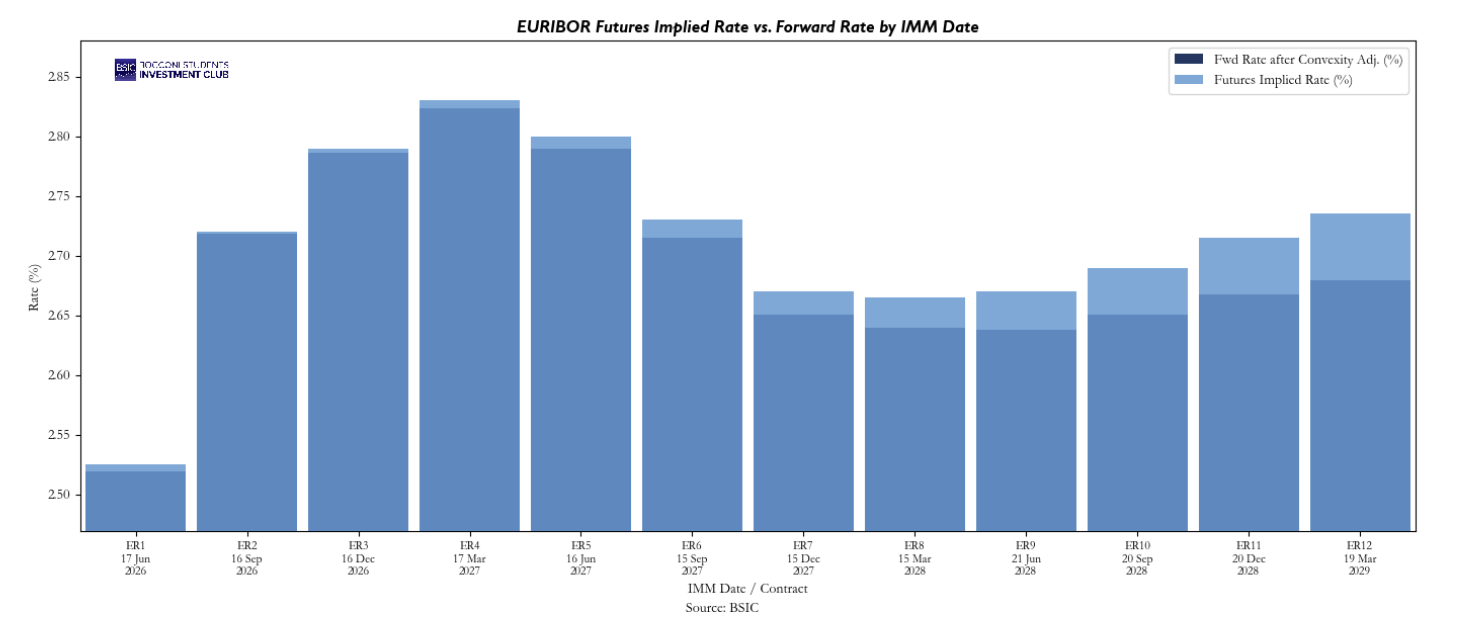

The single free parameter in the Ho-Lee model is σ, the constant short-rate volatility. As this paper focuses on EURIBOR futures as its primary instrument, we calibrate σ to the 2-year ATM normal (basis-point) implied volatility of EUR interest rate caps, which stood at 105.86 bps per annum as of 25 March 2026. This expiry sits comfortably within the ER1–ER12 strip and avoids the distortions that can affect very short-dated caplet volatilities, making it a natural and representative calibration point. The resulting convexity adjustments across the strip are shown above.

Extending the Ho-Lee with Mean Reversion

While the Ho-Lee model produces the elegant closed-form result $\sigma^{2}T_{1}T_{2}/2$ , it rests on two assumptions that limit its theoretical accuracy. First, the short rate volatility $\sigma$ is constant across all maturities, implying that a caplet expiring in three months and one expiring in three years have identical implied volatilities which is a restriction the market cap volatility surface systematically contradicts. Second, the model contains no mean reversion mechanism, leaving the short rate free to wander arbitrarily far from its current level and thereby overstating the convexity adjustment at longer maturities.

Hull and White address both shortcomings by introducing a single additional parameter, the mean reversion speed $a$ , transforming the Ho-Lee dynamics into:

$dr(t)\, = \,\left\lbrack \theta(t) - ar(t) \right\rbrack dt + \sigma dz$

The term $- ar(t)$ acts as a restoring force, pulling the short rate back toward equilibrium. When $a = 0$ the dynamics reduce exactly to Ho-Lee, confirming that Ho-Lee is a limiting case of Hull-White. As before, $\theta(t)$ is determined from today’s forward curve, ensuring exact fit to the initial term structure.

Mean reversion modifies the bond price dynamics in one critical way. Under Ho-Lee the bond’s sensitivity to short rate shocks was $(T - t)\sigma$ which is linear in time to maturity. Under Hull-White this becomes $B(t,T)\sigma$ , where:

$B(t,T) = \frac{1 - e^{- a(T - t)}}{a}$

This function grows with maturity but at a diminishing rate, reflecting the fact that mean reversion limits how far the short rate can drift before the bond matures. $B(t,T) \rightarrow (T - t)\ as\ a \rightarrow 0$ , recovering Ho-Lee exactly. Following the same derivation steps as before, Itô’s Lemma on the log bond price, differencing to obtain the forward rate SDE, and integrating the drift, but with $B(t,T)\sigma$ replacing $(T - t)\sigma$ throughout, the closed-form Hull-White convexity adjustment is:

$CA\left( T_{1},T_{2} \right)\, = \,\frac{B\left( T_{1},T_{2} \right)}{T_{2} - T_{1}}\left[ B\left( T_{1},T_{2} \right)\left( 1 - e^{- 2aT_{1}} \right) + 2aB\left( 0,T_{1} \right)^{2} \right]\frac{\sigma^{2}}{4a}$

where $B\left( T_{1},T_{2} \right) = \frac{1 - e^{- a\left( T_{2} - T_{1} \right)}}{a}$ and $B\left( 0,T_{1} \right) = \frac{1 - e^{- aT_{1}}}{a}$ . As shown in the previous section, this formula reduces to $\sigma^{2}T_{1}T_{2}/2\ as\ a \rightarrow 0$ , confirming the theoretical consistency between the two models.

The Hull-White formula produces smaller convexity adjustments than Ho-Lee at every maturity for any $a\, > \, 0$ . This follows directly from the fact that $B(t,T)$ grows more slowly than (T−t), dampening the bond price’s sensitivity to short rate shocks and reducing the drift accumulated in the forward rate SDE. At short maturities the two models are nearly identical since $B(t,T) \approx (T - t)$ when $a(T - t)$ is small. The divergence grows progressively toward the back of the strip, making the model choice most consequential precisely where the convexity adjustment is largest, which is in the red and green contracts. Using the simpler Ho-Lee adjustment beyond two years will therefore systematically over-correct the futures rate.

Unlike Ho-Lee, where σ is read directly from the flat caplet vol surface, Hull-White requires fitting two parameters jointly. The model-implied ATM normal caplet volatility at expiry T is given in closed form as:

$\sigma_{HW}(T) = \sigma\frac{B(0,T)}{T}$

One calibrates a and σ by minimizing the sum of squared differences between model and market caplet volatilities across the available expiry strip. The mean reversion speed a is identified by the slope of the vol surface and a steeper decline in implied vol with expiry implies a higher a, while a flat surface drives the calibration toward the Ho-Lee limiting case. The two models therefore form a natural hierarchy: Ho-Lee when the vol surface is approximately flat, Hull-White when it has a pronounced term structure.

Comparison of Rates

To construct the observed futures–forward spread, we begin by bootstrapping the EURIBOR 3m swap curve into discount factors, and then extracting forward rates corresponding to the exact IMM dates of the futures contracts. Because market quotes are only available at discrete maturities, we apply log-linear interpolation on discount factors to obtain values at the specific IMM dates to ensure consistency with no-arbitrage principles, although it assumes a constant forward rate between these dates From these interpolated discount factors, we compute the implied forward rates and compare them directly with the corresponding quarterly futures-implied rates, forming the spread $r_{fut} - r_{fwd}$ for each contract.

We then add the convexity adjustment derived from the Ho–Lee framework to the interpolated forward rates, thereby obtaining convexity-adjusted forward rates that are directly comparable to futures rates. The need for interpolation arises because futures contracts reference specific IMM dates that generally do not coincide with quoted curve maturities, making it necessary to construct internally consistent forward rates at those exact dates. Finally, we compare these convexity-adjusted forwards to rates implied by FRAs and examine deviations in the futures–forward spread.

The residual $r_{fut} - r_{fwd}$ is an interesting quantity to examine. If the Ho-Lee adjustment is correctly specified, it should in theory be stationary and centred around zero, as any persistent deviation would imply a systematic mispricing between two instruments referencing the same underlying rate. Empirically testing whether this holds, and whether the residual exhibits mean-reverting behaviour across different volatility regimes, would be a natural extension of this analysis. If stationarity holds, the residual could in principle serve as a relative-value signal between the futures and swap markets. A promising direction for future research would be to repeat this exercise under the Hull-White framework, where mean reversion is expected to reduce the residual at the back of the strip, and to assess whether the more sophisticated calibration meaningfully closes the gap. Multi-factor or stochastic volatility frameworks could be explored further still, particularly for longer-dated contracts where the single-factor Gaussian assumption becomes hardest to defend.

Conclusion

The convexity adjustment discussed above is often derived under simplifying assumptions about the dynamics of interest rates. A common starting point is the Ho-Lee model, which assumes that the short rate follows a simple arithmetic Brownian motion with constant volatility and no mean reversion. This framework is attractive because it yields a closed-form expression for the convexity bias and provides clear intuition: the adjustment increases with the square of volatility and with the time to maturity. However, the Ho-Lee model may ultimately be too simplistic to accurately capture real-world dynamics as it assumes no mean reversion, constant volatility and unbounded rate behaviour.

A more realistic framework is Hull-White which extends Ho-Lee by introducing mean reversion. Implementing this in practice requires estimating mean reversion speed and volatility, whereas Ho-Lee has $a = 0$ and a constant volatility. These parameters can be obtained via regression or bootstrapping. In the future, we could consider adding time-varying volatility and exploring this bias with other STIR futures.

References

Aikin, Stephen, “STIR FUTURES – Trading Euribor and Eurodollar Futures”, 2012
Tuckman, Bruce, Serrat, Angel, “Fixed Income Securities – Tools for Today’s Markets”, 2012
Hull, John, “Options, Futures, and Other Derivatives”, 2014

Published by BSIC on 29 March 202629 March 2026

0 Comments

Leave a Reply Cancel reply

Market Recap 29/03/2026

Risk Neutral Density Estimation from Option Prices

Market Recap 08/03/2026