The aim of this article is to give a quick taste of how it is possible to build practical codes in Python for financial application using the case of Value at Risk (VaR) calculation. The following paragraph will present a brief introduction to Python, then the article will continue with a broad overview of VaR without going into the details of its mathematical properties and then it will tackle different VaR formulas, explaining the main intuition behind and presenting the relative codes. To benefit the most from this article the reader should be already at least vaguely familiar with the concept of Value at Risk, even better if also aware of the diverse mathematical properties of different VaR formulas.
Why Python?
As cited in the official documentation on www.python.org:
“Python is an interpreted, object-oriented, high-level programming language with dynamic semantics. Its high-level built in data structures, combined with dynamic typing and dynamic binding, make it very attractive for Rapid Application Development, as well as for use as a scripting or glue language to connect existing components together. Python’s simple, easy to learn syntax emphasizes readability and therefore reduces the cost of program maintenance.”
Historically there have often been different and diverse roles inside a financial company, specifically both the classic code developer and the employee with a finance background have been present and have been working together on finding a technological solution to perform finance related tasks. This implies that at first one would have to sketch a code in an easy to learn language and then the developer would have to rewrite the initial idea in an efficient way, using a faster and more complex programming language. Unfortunately this process has often implied that the developer, not coming from a financial background, didn’t really understand the original idea in the code and possibly made some mistaking during the process of improving the code while translating it or just rewriting it. Nowadays some programming languages exist that are both fast and easy to learn so that one person can directly code the initial idea without the need of a professional developer to rewrite it. This obviously jumps over possible mistakes arising from communicational misunderstanding or poor knowledge coming from the developer or the other employees.
Python is one of those languages. Thanks to its speed and easy semantics is in fact nowadays prominent in the finance industry, and its success just keeps growing. To learn more about Python and on why it is a great tool for finance follow the links below.
- https://www.python.org/doc/essays/blurb/
- https://www.safaribooksonline.com/library/view/python-for-finance/9781491945360/ch01.html
Value at Risk, brief introduction
Value at risk (VaR) is a certified achievement in the study of quantitative risk management and even if with time its use is increasingly often being combined with other measures of risk, it is still present, in different forms, in the agenda of all market risk managers. Its general form can be written as:
![]()
Where rα is the VaR, hence that loss value for which probability of losses bigger than VaR itself is equal to α. Despite various critiques concerning the inability of VaR to measure the magnitude of losses over α, it remains a key element in financial risk management and for such reason its calculation is still very important.
There are multiple techniques to calculate VaR with differences in formulas and sampling, strongly altering their ability to foresee future risks and to shield the asset manager from possible downsides, It is therefore of utmost importance to understand the general differences among them. In the next section a brief introduction to the main characteristic of four different VaR formulas is given and the relative Python code on how to build them is presented.
VaR – one function for four formulas
An alternative and more precise solution to download the full code is to visit this GitHub repository where the code is held:
This first section contains the importing of the necessary libraries, the definition of a function that will contain all the different formulas and parameters setting, and some initial settings to handle missing inputs. In every sub-formula there will be a distinction between a call for a single VaR referring to the last period interval, and a call for a series covering the whole set of data.
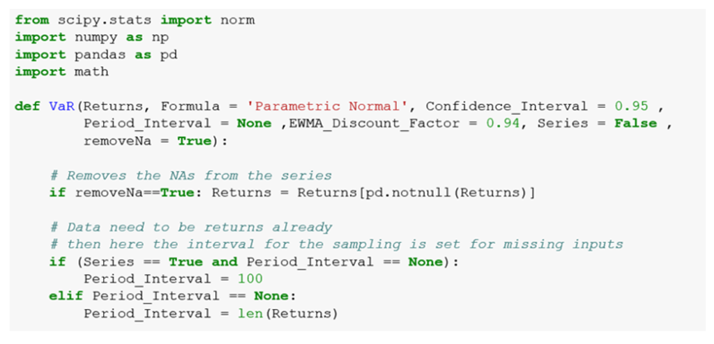
Source: BSIC
Parametric VaR (Variance/Covariance VAR) is the most common form used in practice due to its simple nature and the low number of parameters it requires to be computed. To build it, the only variables needed are the mean and the standard deviation of a portfolio/security. The problem that follows from such simple requirements is that it works under two restrictive assumptions, namely normal distribution and independence of returns. This leads to myopically equating all returns in terms of importance, overlooking big shocks that should be carried over and should be given more power to impact the actual VaR. It is possible to notice, in fact, that the parametric method is one of the most stable among the presented VaR formulas, highlighting its lack of capability to absorb new information and shape the capital risk appropriately.
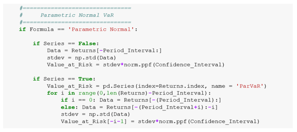
Source: BSIC
EWMA (Exponentially weighted moving average) is a step forward from the parametric VaR, in the sense that it tries to solve the problem of slow reaction to new information and the equal importance of returns. Using a decay factor the EWMA formula is able to weight different information as it comes in, giving more importance to recent returns and less importance to data far in the past by slowly decaying their contribution to the VaR. Through this, the measure limits the ‘echo effect’, occurring when a large shock of the past becomes too old to be considered and leaves the estimation, causing a big change in the VaR which is not due to a change in the markets.
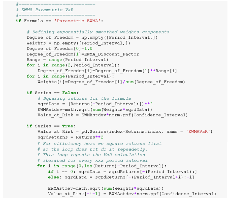
Source: BSIC
Historical Simulation (HS) VaR is instead efficient when the risk manager cannot, or doesn’t intend to, make assumptions on the underlying distribution of returns as it is calculated by the simple picking of the chosen percentile loss in a given period of time. This method is even simpler than the parametric one and that is precisely its weakness. The main underlying logic is that the past is a good predictor for the future. By looking back, it is then possible to incorporate all data points into the risk calculation but this unfortunately leads to too simplistic a model.
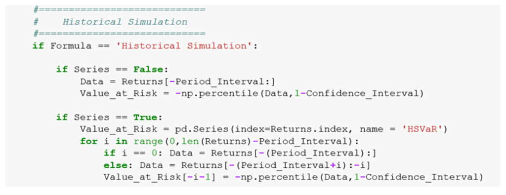 Source: BSIC
Filtered Historical Simulation VaR can be described as being a mixture of the historical simulation and EWMA methods. Returns are first standardized, with volatility estimation weighted as in EWMA VaR, before a historical percentile is applied to the standardized return as in the historical model. From the graphs it is easy to spot that this model looks very much like EWMA, as returns are standardised and weighted by the same decay factor. The main difference lies in the fact that this model is generally more conservative because it looks at the worst past losses and adjust its VaR value according to it.
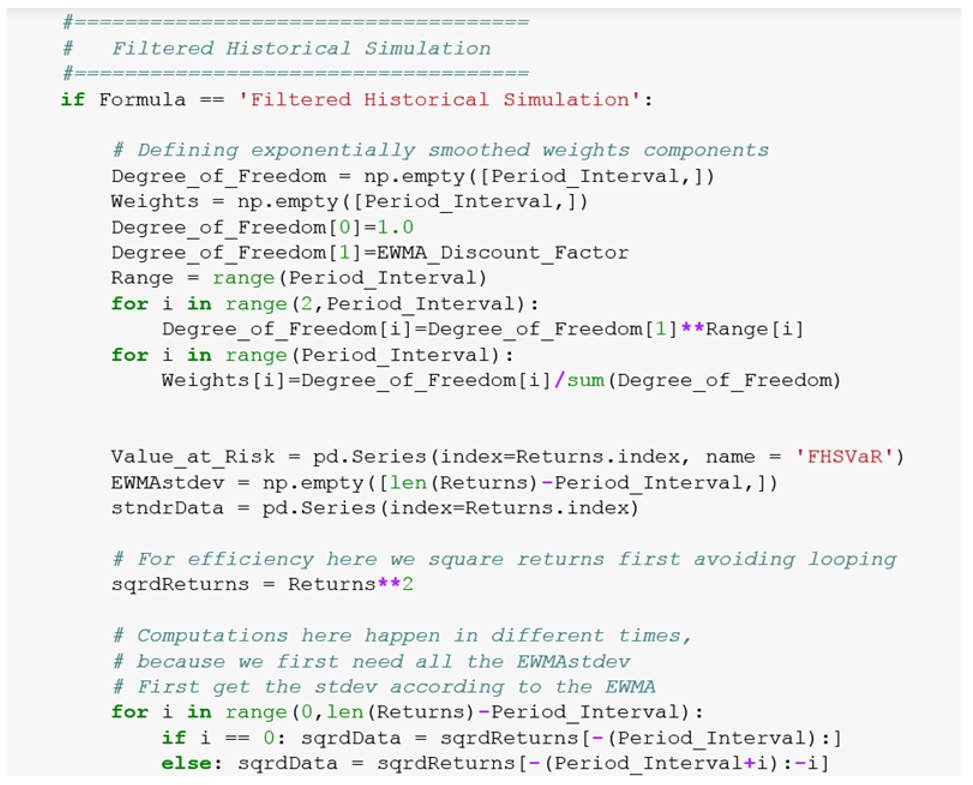
Source: BSIC
Source: BSIC
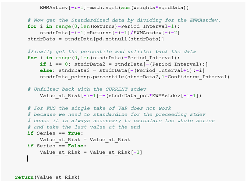
The last line closes the initial ‘def’ statement and returns the requested VaR calculation.
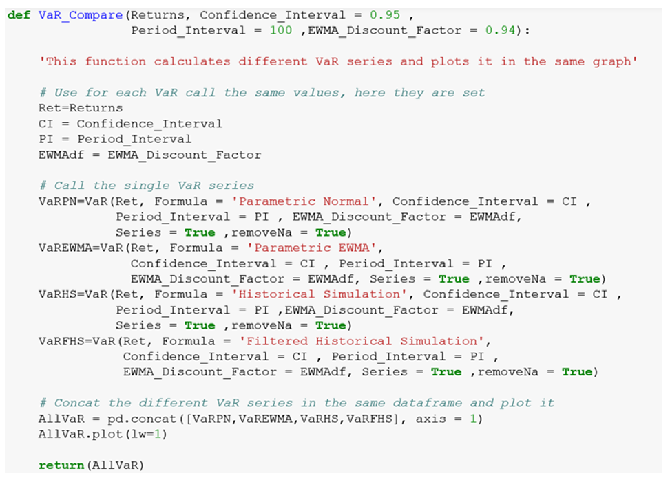
VaR_Compare – let us see the differences
The next function is just a wrapper that calls the previously defined VaR function four times, each with a different formula, wraps the VaR series in one datasets and then plots it in a chart.
Source: BSIC
An example results using VaR_Compare on a series of an ETF’s daily returns:
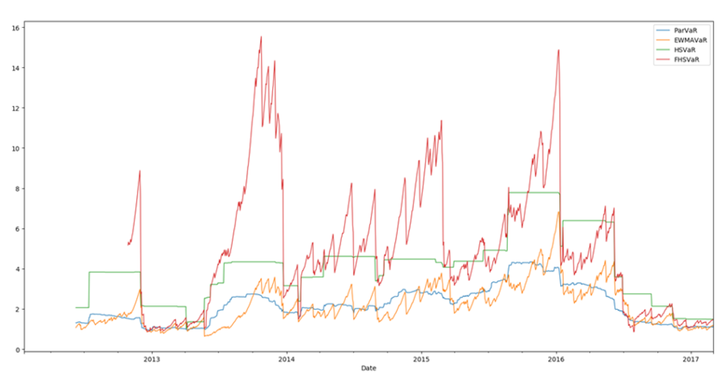
Chart 1: Plot of VaR_Compare
Source: BSIC


0 Comments