The famous Black-Scholes model is a mathematical model used for pricing financial derivatives. It is particularly useful because it offers an explicit formula for the value of a European option in terms of time to expiry of the contract T, risk-free interest rate r, strike price of the option K, price of the underlying at time t=0 S0 and volatility of the underlying σ. For instance we can write the value of a call option C as C=BS(S0, K, σ, t, r). The model is based on several assumptions, such as frictionless market and absence of arbitrage opportunities, but here we will focus on two of them: that the time evolution of the price of the underlying follows a geometric Brownian motion and that the volatility of this motion is constant.
Practically, the first statement means that at time t=0 the price of the underlying is S0, at time t=T the logarithm of its value ln(ST) is a random variable which follows a normal distribution with mean
Log(S0)+(μ-σ²/2)T
and variance
σ²T
where μ is the expected return on the underlying. This property of ST is called log-normality.
For a contract in an economic system S0, K, T and r are known but σ is not determined, as it is different from the historical volatility, that is the one realized in the past. However, we can infer the volatility σimplied which is needed so that the value predicted by the BS model corresponds to the market price of an exchange traded option Cmkt with the same parameters.
C=BS(S0, K, σimplied, t, r)
This volatility is called implied volatility or IV, as it is implied in the market price of the option.
Although we assumed the volatility to be constant, if we measure the IV for different strike prices and different exercise time, we will find them to be anything but constant. In particular, the two common patterns emerge: the smile and the skew.
The volatility smile is typical of options whose underlying is a foreign currency. As shown in Fig. 1.a, the IV for at-the-money call options (ATM, those for witch S0≈K) is lower than the IV for the out-of-the-money and in-the-money call options (OTM and ITM, respectively when K>S0 and K<S0).
On the other hand, the volatility skew concerns options on stocks or stock indexes. As in Fig. 1.b, IV decreases with the increase of the strike price, which means that the volatility used to price an ITM call is higher than the one used to price an OTM call on the same underlying. This pattern was less pronounced before the stock market crash of October 1987. This fact suggests that one cause at the origin of the skew could be the fear of financial crisis, because the OTM put option (for which S0>K) is a cheap protection against equities fall and their high demand would make them overpriced.
Another explanation regards the other assumption we made at the beginning: log-normality. The variation in volatility reflects the fact that the probability density distribution f of ln(ST) is not normal. Here are some examples.
The first graph (Fig. 2) shows three hypothetic IV smiles. As the IV curve tends to follow the movement of S0 (it shifts to the right if S0 increases and vice versa), it is plotted with respect to ln(K/F0), where F0=S0erT on the x axis. For each smile that has been calculated, its curvature is the mean of the inverse of the radius of curvature along each curve. Using the same parameters S0, r, T we can calculate the price of a call option in terms of K (Fig. 3).
C(K)=BS(S0, K, IV(K), t, r)
The following step is to obtain the probability density function from the option prices. We can obtain the risk-neutral probability measure in the following way.
First of all, the risk-neutral probability measure frisk neutral is equivalent to the condition of no-arbitrage and is the probability measure in a risk-neutral world (usually investors are risk averse). It can be demonstrated that the value of an asset is the present value of its expected pay-off under the risk-neutral probability measure. Indeed, for a call option:
After deriving twice the option value with respect to the strike price, we can easily obtain frisk neutral.
If ST followed a lognormal distribution, accordingly to frisk neutral, Log(ST) would be distributed as
In Fig. 4, is plotted for each of the initial different IV smiles. As we can see, as the curvature of the IV curve increases, the kurtosis of frisk neutral increases as well. Kurtosis is a descriptor of the shape of the density function. A distribution with higher kurtosis has got higher probabilities in the central values and in the more extreme. This characteristic, known as fat tails, means that this extreme events are more likely to happen and, because they include huge losses, they are a sign of increased risk. In Fig. 5 we can see the direct relation between the kurtosis of the probability distribution and the curvature of parabolic IV smiles like the ones previously described.
Now we consider the IV skew. The procedure is the same as before: we assume a IV curve following the pattern of a skew (Fig. 6) with three different curvatures, from which we obtain the call option prices (Fig. 7). The second derivative gives us the risk-neutral probability density function (Fig. 8). As before, kurtosis increases with the IV curvature. One interesting feature is the decrease of the skewness. The skewness is a measure of the asymmetry of the distribution. Negative skewness means that the tail on the left of the distribution is longer or fatter, which means that lower outcomes are more likely than higher ones. As the left tail represents losses in the value of the asset, the curvature of the IV skew is a signal of increased risk. In fact, declines in the S&P 500 are followed by rises in the steepness of the IV curve.
In the last part, we will apply the method used before to obtain the risk-neutral measure from market data. We consider call options on the S&P 500 index with different strike prices and maturities. Let’s start with the option ending on the 16th June 2017. First of all, we should not consider illiquid contracts deep ITM and OTM. Then we use the mean between the bid and the ask price to obtain the IV in terms of ln(K/F0) (where F0=S0erT) and use a spline interpolation with the values we have found (Fig. 9.a). The purpose of the spline is to smooth the curve and to interpolate more values for the strikes between the one traded. Each couple of values (IV,K) so obtained is used to calculate the price of the relative call option using the BS model (Fig. 9.b).
The graph in Fig. 9.c is obtained. The distribution is clearly non normal: it is negatively skewed by -0.05487991. As we avoided illiquid contract deep ITM and OTM, the graph misses the two tails. We can extend the tail using a polynomial extrapolation on both sides (Fig.10). The green line is a normal distribution with the same mean and variance of the one obtained from the IV curve. It is straightforward to appreciate the difference between the distribution just obtained (with skewness = -0.7330008 and kurtosis = 3.2817684) and the normal one (with skewness=0 and kurtosis =3).
Comparing different maturities, we can plot a graph of the implied volatility depending on both strike price and maturity. The following graphs (Fig. 11 and Fig.12) show the data from contracts ending in December, January, March and June. In particular, we can notice that since the curvature of the surface diminishes for longer maturities, the kurtosis of the probability density decreases as well (the central peak of the distribution is lower and wider from left to right in the graph).
[edmc id= 4292]Download as PDF[/edmc]


0 Comments