Introduction
In this article, together with a brief introduction to the use of option-implied information in forecasting, we would like to give an answer to the question: does Option-Implied Skewness and Kurtosis improve the predictive power of (Squared) Implied Volatilities on Future Realised Variance? In order to do so, we will analyse existing literature on the forecasting power of Black-Scholes Implied Volatility (BSIV) and, by using both “expanded” Black-Scholes (i.e. the “Jarrow-Rudd” pricing formula) estimates as well as model-free (i.e. the “Option Replication Approach”) estimates of option-implied Variance, Skewness and Kurtosis, we will assess whether the option-price higher moments are a better predictor than the BSIV squared alone.
The Use of Derivatives in Forecasting
A derivative contract is an asset whose future payoff depends on the uncertain realization of the price of an underlying asset. Many different types of derivative contracts exist: futures and forward contracts, interest rate swaps, currency and other plain-vanilla swaps, credit default swaps (CDS) and variance swaps, collateralized debt obligations (CDOs) and basket options, European style call and put options, and American style and exotic options. Several of these classes of derivatives, such as futures and options, exist for many different types of underlying assets, such as commodities, equities, and equity indexes.
Theoretically, from all these types of financial derivatives it is possible to extract some information. However, practically speaking, this is feasible only for those securities where the market is sufficiently large and liquid in order to avoid the information contained in the derivatives prices to be distorted by the presence of large liquidity premia (in other words, the price of an illiquid, customized derivative is likely to be “high” as the dealer requires a compensation for selling a structure which can be only partially hedged through other traded derivatives). Moreover, in an illiquid market, the value of a contract might not change even in the presence of new information simply because the product does not trade at all and thus no new prices are available for that security. It is therefore much preferable to stick with “vanilla” derivatives rather than exotic and bespoken structures. Another reason for this is given by the fact that some “exotic” derivatives have path-dependent payoffs which makes the extraction of information extremely complicated.
At the same time, Delta-1 derivatives, i.e. the ones whose value increases or decreases in a linear fashion as the underlying price changes, such as Futures and Forwards, provide much less information than other derivatives which are characterised by a non-linear payoff function. The reason being that derivatives with Percentage Delta (Δ%) equal to 1, have no optionality and the price of those securities is a simple linear function of the underlying asset price and therefore information contained in these prices is unlikely to be more useful than the underlying price itself. We are thus looking to extract valuable information from derivatives who are non-linear in their payoff and for whom a large, developed and liquid market exists. The natural candidates for this are “plain vanilla” options, i.e. simple put and call options. Focus should be on European-style contracts as the possibility of early-exercise (which is the defining characteristic of American-style options) does alter the value of the contracts and thus, the information that we would extract from them – however the reader should note that, given the price of any American-style contract, it is possible to derive the early exercise premium and, by subtracting the latter to the market value of the derivative is possible to get the price of the corresponding synthetic European derivative.
One note: among vanilla options, it is much easier to deal with stock-index options than single-stock options. This is due to various reasons but we would tend to say that the main one is related to the discrete cash dividend payments of single stocks (if any) and the associated (anticipated) “jump” in its price on the Ex-Dividend date. In fact, whilst professional data platforms, such as Bloomberg, provide the user with a time series of the stock-price that corrects for the dividend payment, it is quite cumbersome to filter the effect of discrete dividends from option-implied volatilities.
Forecasting with option-implied information is a process that can be separated in two steps: in the first, derivative prices are used to extract the relevant aspect of the option-implied distribution of the underlying asset whilst in the second an econometric model is used to relate this option-implied information to the forecasting object of interest. For the reader who wishes to dive further into the use of option-implied information in econometrics we would suggest to look at: Garcia et al. – The econometrics of option pricing.
Regarding the first step, which is the core of this article, whose main reference is Christoffersen et al. – Forecasting with Option-Implied Information, we would like to point out that extracting information out of option prices can be done through different techniques that belong to two distinct families: model-dependent and model-free estimation techniques.
To summarise, the key point of this paragraph is that derivatives prices contain information useful to forecast any twice differentiable function of the future underlying price. However, some derivative contracts are linear in the return on the underlying security and therefore their payoffs are too simple to contain useful information whilst other derivatives contain information whose extraction is too cumbersome. Therefore, we will focus on European-style vanilla options on the most liquid Equity Indexes, as most of the literature does.
Black-Scholes Model Misspecifications
For a detailed (but very easily understandable) treatment of the Black-Scholes formula, its derivation and implementation in VBA as well as basic Greeks, please see: https://bsic.it/black-scholes-model-vba/. For a detailed treatment of higher order Greeks for vanilla options please see: https://bsic.it/guide-land-higher-order-greeks/. For a general introduction to Volatility please see: https://bsic.it/let-volatile/ whilst for an explanation of cross-movements of the volatility skew please see: https://bsic.it/riding-volatility-surface/
The Black-Scholes framework is very convenient in the sense that it is a single-factor model, meaning that the formula has just one unobserved parameter, that is, volatility (“sigma”) which can be easily obtained for any option with a market price. In the article we will call BSIV – Black Scholes Implied Volatility, the value of sigma that, once plugged into the BS pricing formula (together with contract-specific and other directly observable parameters such as the interest rate) will return the observed market price of the option.
It is well-know that Black-Scholes model is not a representative model of reality: in fact, returns are not normally distributed and volatility is not constant over time. The former can be easily proven by the presence of the “Volatility Skew” (or “Smirk” or “Smile”), that is, prices of options with the same maturity but different moneyness do incorporate different levels of (Black-Scholes) Implied Volatility, whilst the latter statement can be understood by observing that options with the same (spot and forward) moneyness but different maturities are pricing different level of annualised volatility; translation: Implied Volatilities have a term-structure (that can be either downward-sloping or upward-sloping) and this makes the BS assumption of constant volatility over time unrealistic. We can thus say that Black-Scholes model is a mis-specified one.
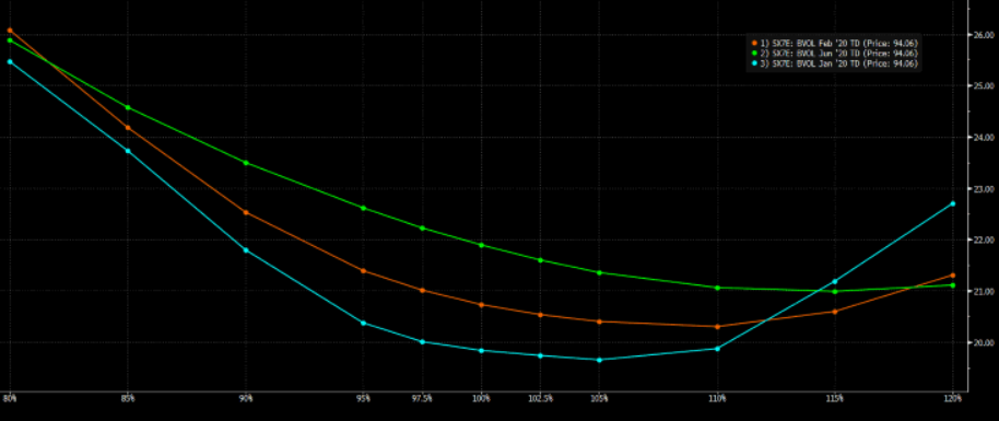
An example of the Volatility Skew for three different Contract Maturities – Source: Bloomberg
Because of the model mis-specifications (and, as a lower magnitude effect, the presence of risk premia), we can conclude that BSIV does not reflect the “true” Expected Volatility, that is, BSIV squared is not a true measure of Expected Variance. If we assume that the “marginal” market player is, on average, right in her expectations, we can intuitively conclude that BSIV is not an unbiased estimator of future realised volatility (and existing literature on the topic indeed does confirm this statement). An equivalent but easier statement is that deep-OTM Put options are more expensive than what BS suggests and, at least in “quiet” times, BSIV for ATM contracts tends to be larger for longer maturity contracts.
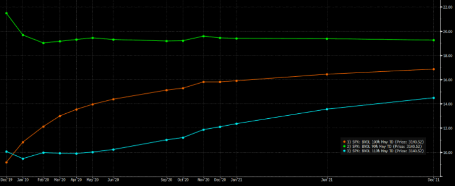
An example of the IV Term Structure for three different Moneyness (orange = ATM) – Source: Bloomberg
Given what has been said so far shall we throw away the Black-Scholes models and the BSIV? Absolutely no. In fact, as we will shortly see, “simple” BSIV is a better predictor for the future volatility of the underlying asset than historical measures of (past) volatility.
Is there any other model beyond Black-Scholes? Yes, the most important being the Heston model and the generic class of jump-diffusion models. Although these models represent a big improvement from the simple BS framework (for instance, the Heston model allows for non-constant, mean reverting volatility and correlated innovations in the underlying price and its volatility), as long as the “mere” volatility forecasting is concerned, BSIV is still preferred to the estimates obtained through these more complex models.
Another possible alternative to BSIV is given by Model-Free Implied Volatility (in short, MFIV). However, it is worth noting that existing literature does not agree on which one among BSIV and MFIV works better as a predictor for future realised volatility, with different studies obtaining opposite results.
To sum up, the (very basic) key takeaway from this paragraph should be that any traded option has a price. That price, which represents the amount of money that investors are willing to pay (receive) to buy (sell) the contract, can be univocally associated to a certain BSIV (by inverting the Black-Scholes formula). However, since BS assumptions do not hold and the market prices risk premia, BSIV is not the “true” expected future volatility and, as the distribution of returns is non-normal, the price of options will be given by market agents’ expectations about the density function of future returns, that is, investors’ beliefs on higher moments of the distribution of returns. This implies that from option quoted prices it is possible to obtain option-implied expected variance, skewness and kurtosis of the return distribution, as well as the whole PDF. In simpler terms: two options (same moneyness and same maturity) written on two different stock indexes (with the same drift) will have a different price (and thus two different BSIV), even if the return distributions of the indexes are identical up to the first two moments, because of different Skewness and/or Kurtosis. Even more intuitive: option prices do incorporate expectations about the asymmetry and leptokurtosis of the return distribution – however these are not captured by the BS formula which “pushes” these factor into biased values of BSIV.
In the latest part of this article we will assess whether using different measures for the three (implied) moments (Variance, Skewness, Kurtosis) allows us to predict future RV better than BSIV, both as standalone variables as well as together with historical measure of (past) Realised Variance (whose predictive power is, ex-ante, justifiable by the well-known Volatility Clustering phenomena).
Literature Review
In this section we would like to present some results concerning the use of Option-Implied information in forecasting. The main reference, together with the already mentioned Christoffersen et al. which briefly describes the result of several studies in the field, is Busch et al. (2011) – The role of implied volatility in forecasting future realized volatility and jumps in foreign exchange, stock, and bond markets. We focus on the results of this paper as it is the one that provided the most compelling evidence in favour of BSIV squared as a predictor for future Realised Variance. Moreover, in our own empirical study, which will be presented in the second part of the article, we will use a similar (albeit easier) approach to assess whether decomposing option prices into three components (Variance, Skewness, Kurtosis), rather than simply using BSIV squared, improves the forecasting power of the regression.
Busch and co-authors use derivative prices and investigate whether implied volatilities (IV) backed out from options on foreign currency futures, stock index futures, or Treasury bond (T-bond) futures contain incremental information when assessed against volatility forecasts based on high-frequency (5-min) current and past returns on exchange rates, stock index futures, and T-bond futures, respectively. That is, they regress total Realised Variance (RV) for the current month on the lagged monthly (subscript M), weekly (subscript W) and daily (subscript D) Realised Variance. Black–Scholes Implied Variance (BSIV^2) is introduced in univariate regressions as well as an additional regressor in the RV. They find that the latter outperforms past Realised Variance as a predictive tool. Also, they compute an alternative volatility measure which separate Realised Variance (RV) into two components, the Continuous-Sample Path component (C) and the Jump component (J). They find that the predictive power of lagged realised variance is higher when this is decomposed into these two dimensions. However, a univariate regression on squared BSIV still outperforms the regression on decomposed Realised Variance.
The best results (from the Adjusted R^2 maximisation point of view) are obtained by regressing Realised Variance on the decomposed lagged RV (that is, by the regression on C, J, BSIV^2). However, the out-of-sample test reveals that MAFE (Mean Absolute Forecast Error) is minimum if the regression of RV is performed only on BSIV^2. Results from Busch et al. (2011) are summarised in the following table.
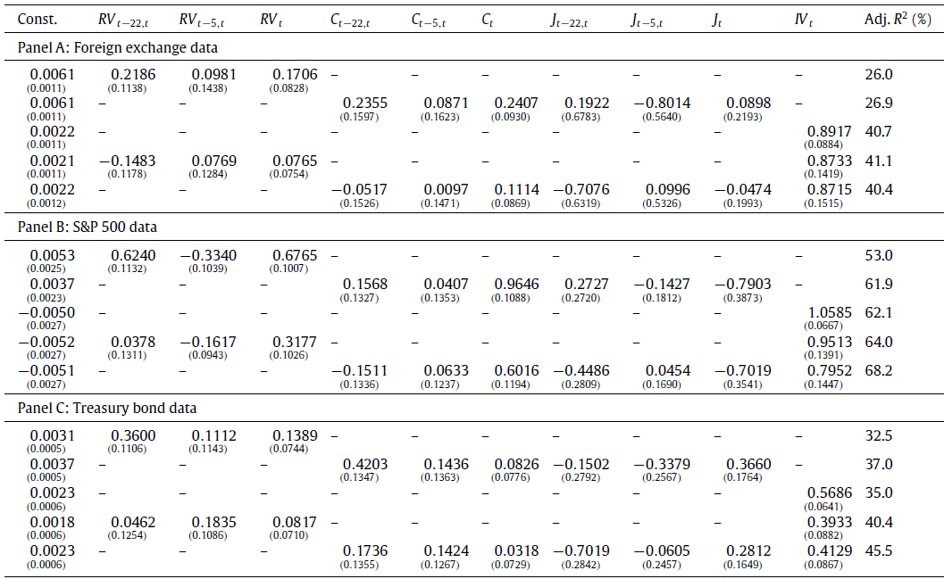
Source: T. Busch et al. / Journal of Econometrics 160 (2011) 48–57
As we can see, for all the three markets the Adjusted R^2 is higher if BSIV^2 is included among the regressors although the goodness of fit of the model depends on the asset class: in fact, Black-Scholes Implied Variance is able to explain only 35% of the RV for Treasury Bond Futures and 40% for the FX whilst for SPX the portion of variance explained by BSIV^2 alone is almost 65%.
The Next Step
In the following part of the article we will present the mathematical tools that we will need to extract information about higher moments of the (expected) Risk Neutral Returns distribution that is implied in options prices. Particularly we will present both the Jarrow-Rudd pricing formula (which is a model-dependent expansion of Black-Scholes) and the Option Replicating Approach (which is model-free). We will then use these higher order moments in the regression of Realised Variance and we will compare the results with the one obtained by performing the regression only on BSIV^2. Finally, we will check whether using a second-order polynomial interpolation to create additional (artificial) option prices (thus increasing the number of strikes used in the computation of higher order moments) will generate any improvement in the forecasting power of the regression on RV.


0 Comments