Inflation Derivatives and the Inflation Risk Premium – Part 1

“Inflation is when you pay fifteen dollars for the ten-dollar haircut you used to get for five dollars when you had hair”

Sam Ewing

Inflation is an elusive phenomenon which is sometimes dubbed a “hidden tax”, eroding purchasing power and returns.

This article is the first in a series of two. In this first part, we are going to give an overview of inflation derivatives and present some intuitions for their pricing. The second part, due next week, will analyse the inflation risk premium and its dynamics in light of recent monetary policy developments.

What is inflation?

Inflation is usually defined as “the tendency of prices of consumer goods and services to increase over time”. In other terms, as prices increase, the amount of goods that one unit of currency can buy decreases over time, thus reducing the purchasing power of economic agents. It is reasonable to assume that agents do not care in holding money per se, but only insofar as they can exchange money for goods and services. It follows that investors will focus on real returns, i.e. nominal returns adjusted for the relevant inflation rate, and will, therefore, take steps to limit and hedge inflation exposures.

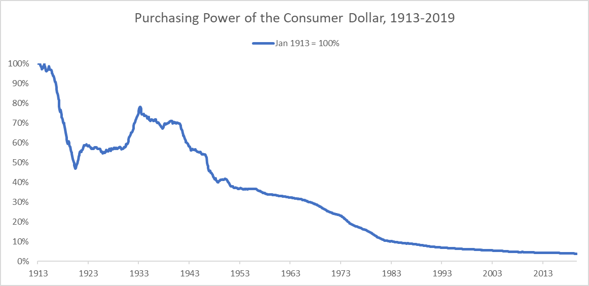
Source: FRED

How is inflation measured?

Since economic agents are interested in different goods the value of money is, to a certain extent, subjective. This is clearly an issue when trying to find an objective measure for the rate of inflation within a particular market, for instance, a national economy. The standard approach is to focus on a sample basket, which is supposed to be representative of a typical consumer. The methodology for the choice of the basket and its weightings is all but straightforward and, as usual, the devil is in the details. For our purposes, it is enough to say that by choosing a base year for the basket, it is possible to build a price index – the variation of which defines the inflation rates. Sample baskets and index methodologies can vary significantly across countries, as well as time as consumers’ preferences change. Food, housing and transportation usually account for large weights of the index. Seasonal patterns have also a large effect on inflation, and a different treatment of seasonal items can lead to higher variability of inflation indices.

A typical inflation index is the Consumer Price Index (CPI), which is the standard inflation index in most countries. At the European level, the main index is the Harmonised Index of Consumer Prices (HICP), which is a weighted average of indices of members of the Eurozone.

A final point is on rounding practices. Although many indices are now rounded to three decimals, it used to be common practice to round to the nearest decimal. This created two main issues. First, it had an impact when computing percentage changes in inflation, especially relevant in low-inflation regimes. Second, it had a sizable impact on inflation options, as the rounding could determine whether the option would expire in the money or not.

Inflation Linked Bonds

In their modern configuration, inflation securities started appearing in the 1980s in the form of Inflation-Linked Bonds (ILBs). Since then, the market has grown significantly and is now of several trillions in size.

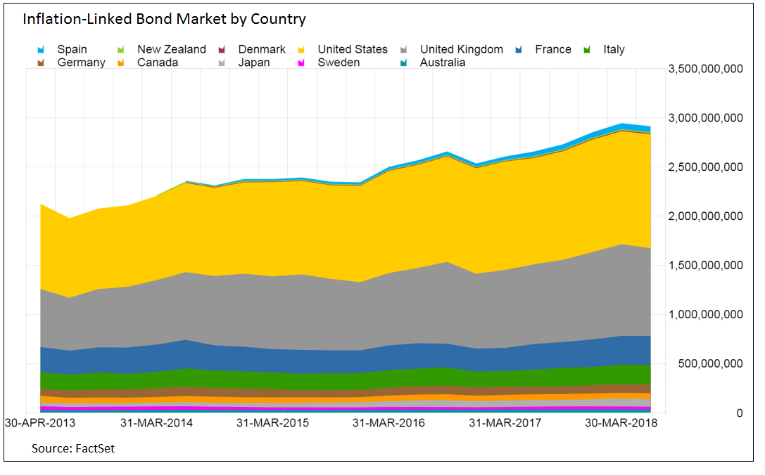
Source: FactSet

As the name suggests, ILBs allow investors to reduce exposure to inflation risk since both principal and coupon payments are adjusted for inflation during the life of the bond. As such, ILBs have uncertain cash flows over their life, which can be broken down in a fixed real component and a variable inflation-linked component.

Why would a government issue such products? First, income from tax revenue is likely to be linked to inflation and thus ILBs allow matching liabilities with future revenues. Second, it gives credibility to economic policy with respect to inflation, since a government will be unable to “inflate” awaits current stock of debt. Finally, there is a strong demand for ILBs, for example by pension funds, which are often under the obligation to pay out inflation-adjusted pensions.

The most basic ILB is the zero-coupon (ZC) ILB. This bond pays a single cash flow at maturity, equal to in nominal units and 1 real unit. Similar to the nominal market there is no issuance of ZC ILBs, but we can easily think of coupon ILBs as portfolios of ZC ILBs with different maturities. It is also common practice to issue these bonds with a minimum guaranteed redemption at par, which in practice means that there is an embedded option providing a hedge against deflation. The pricing and hedging of these inflation floors were among the main drivers behind the development of inflation options.

When dealing with the pricing and trading of ILBs we encounter a problem. Inflation levels are released monthly, usually a couple of weeks after the month under consideration, but of course trading needs to happen daily. To solve this problem a daily reference rate is calculated by linear interpolation using past index values, usually the previous two and three months. This allows traders to quote ILBs in real terms – to get the nominal price one can just use the daily reference rate.

This, however, creates a further problem in that coupon and principal payments are not reflective of current inflation levels but of lagged ones. This effectively means that the investor is without protection for the last period of the bond, usually three months. The investor is partially compensated by the fact that for the first payments he receives inflation payments for periods before the purchase of the bond. While the issue is generally small for coupon payments it can become significant for the final redemption, especially if there is a sudden acceleration in prices during the last period.

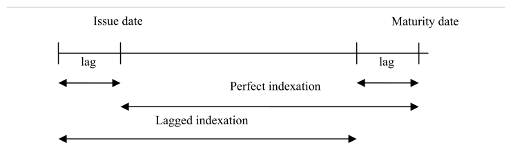
Source: Kerkhof, “Inflation Derivatives Explained”

A key indicator when dealing with ILBs is the Breakeven Inflation rate (BI). This is the inflation rate that would equalise the ILB returns with respect to a similar non-linked bond. Breakeven inflation is usually computed as:

Where and are the nominal and real yields, respectively.

Stated in other terms, BI is the ex-post realised inflation which would make an investor indifferent between the two bonds.

A natural question arises: can we interpret BI as the market expected inflation?

Although the breakeven inflation does incorporate the market consensus for future inflation, there are some confounding factors. First of all, the equality would hold in a risk-neutral world, while investors will likely pay a premium to hold a security with more (real) cash-flow certainty. This premium, conveniently called “inflation risk premium”, will be the subject of further analysis in the second article of this series.

Moreover, ILBs are generally less liquid than their nominal counterparts. This means that they will often carry a “liquidity discount” which works in the opposite way as the inflation risk premium.

There are also a couple of more technical reasons. First, ILBs are convex in inflation changes, which is an attractive feature for investors and thus will likely carry a premium. Second, a compounding effect puts upward pressure on the breakeven inflation, since it can be proven that:

A final consideration is concerning volatility. From the Fisher equation:

We get:

This implies that, if the covariance term is positive (which is generally true empirically), real yields will be less volatile than nominal yields. For this reason, ILBs are generally considered to be less risky than nominal bonds.

Inflation Swaps

One of the basic building blocks of inflation derivatives, a ZC inflation swap is a bilateral agreement to exchange an inflation-linked payment for a non-linked one. The inflation leg pays the net increase in the reference index:

The non-inflation leg can be either fixed or floating. When fixed, it is usually quoted in annualised terms:

As is usual with swaps, the swap rate b is set so that the two legs have equal (expected) present value. With this notation, b is also called the Breakeven Swap Inflation rate, for inflation between and , where can be different than today if the swap is forward starting.

Similar to BI of ILBs, the Breakeven Swap Inflation rate is an imperfect measure of expected inflation. In practice, breakeven rates are often used by central banks and authorities to measure market expectation for future inflation. To mitigate the problems outlined above, it is common to practice to use breakeven inflation to measure changes in inflation expectations, rather than absolute levels. A common choice is the 5y5y inflation swap i.e. the 5-year forward starting 5-year inflation swap.

Finally, ZC inflation swaps are particularly useful because it is possible to derive a model-independent pricing formula and thus strip real ZC bond prices from market quotes.

Inflation options

Initially driven by the need to price and hedge minimum redemption clauses in ILBs, inflation options are another popular instrument to take inflation exposures. These options follow the jargon of interest rate options, where a call (put) option is called a caplet (floorlet) and a series of caplets (floorlets) is called a cap (floor).

As an example, the payoff of a ZC inflation caplet is:

Inflation swaptions are also traded and are usually quoted in the form , where is the expiry and the tenor of the inflation swap.

Pricing inflation derivatives

When pricing inflation derivatives, a few issues arise. First, although there is a large body of literature about inflation modelling, it is often from an “economic” point of view. This means that these models don’t usually say anything about how inflation derivatives should be hedged or about relative values between different instruments, making it practically useless for trading and pricing purposes. Second, interest rates and inflation tend to follow some correlations patters and hence models need to be flexible enough to correctly incorporate these correlations.

During the past decades, two main pricing frameworks have been established.

The foreign market analogy

In this setting, we treat the real and domestic economies as two distinct countries. This means that we have real (domestic) rates and nominal (foreign) ones. The inflation index is then considered the “exchange rate” between these fictitious economies. Following this intuition then, pricing an inflation derivative becomes no harder than pricing a cross-currency interest rate derivative.

Note that there is no redundancy in modelling all three variables in the same model. In this framework, the real rate should be interpreted as the “expected real rate” that we can lock-in using inflation derivatives, the “true” real rate is still unknown.

A common choice is to use the popular HJM framework to model the two interest rates and add a lognormal exchange-rate process for the inflation index. A problem of this approach is in the calibration, which is one of the reasons that led to the development of market models.

Market models

Following the popularity of market models for interest rates derivatives, several authors have introduced market models based on the forward indices. In this setting we model the forward inflation index:

Where is the nominal price at time of a ZC Inflation Linked Bond with maturity T while is the price of a non-linked ZC bond.

Making some assumptions about the evolution of , it is possible to derive arbitrage-free pricing formulas for inflation derivatives. The model can be further expanded, for instance by including stochastic volatility.