Introduction
For the last two years, the large majority of central banks have been hiking rates and conducting quantitative tightening programs to fight against the inflationary pressures witnessed in almost every country after the Covid reopening, supply chain shocks, Russia-Ukraine war, labor shortages, and other related factors. Despite all these efforts, in most of the advanced economies, the results achieved have been quite poor, at least when compared to markets’ initial expectations, with core inflation remaining at elevated levels, well above the central bank’s targets, and the economic activity proving to be extremely resilient. While central bankers have kept referring to “long and variable” lags that can separate the moment these policies are announced from the time when the actual effects on the real economy start to be felt, some commentators are hypothesizing that economies are not responding to the current restrictive policies because of an increase in the natural rate of interest1, also known as r*. This implies that, to obtain the same restrictive effects on the economy and inflation, central bankers would need to take more action than before, with further tightening.
In this article, after analyzing the nature of r*, its importance, and its estimation models, we will discuss how asset classes perform in different r* environments. Similarly, in the last paragraph, we analyze the historical influence of r* on factors’ performances.
What is r*, how is it estimated, and is it rising?
The natural rate of interest, hypothesized for the first time by the Swedish economist Knut Wicksell in 1898, is the real interest rate that supports the economy at its natural level of output while keeping inflation constant. In simpler terms, it is the real rate at which monetary policy is neither accommodative nor restrictive. This means that whenever the actual interest rate is below this value, the economy tends to expand above potential, generating inflation and causing unemployment to decrease below its natural level. On the other hand, when the interest rate is set above r*, the economy tends to contract, inflation shrinks, and unemployment rises. These linked dynamics are what the mandates of all central banks around the world are based on. In fact, since r* is the key parameter to assess the degree of easing or tightening of a certain policy, without having a reasonable estimation of the natural rate, central bankers cannot conduct monetary policies in a responsible way and the risk of massive economic imbalances and crises rises significantly. This argument can be expanded to financial markets. As monetary policy-related decisions have a direct influence on asset classes’ performances, it is logical that r* will play a role in determining asset classes’ returns as well.
Even though this could look elementary, it must be noted that r* cannot be observed directly but needs to be estimated by complex models that take into account macroeconomic, demographic, and social factors. Moreover, r* is believed to be unstable, drifting up or down over time and to vary widely from jurisdiction to jurisdiction. This is one of the reasons why the job of central banks is so complicated, especially when it involves setting a unified policy for a large heterogeneous jurisdiction, like the United States or the Euro Area. The most widely used tools to estimate r* are Laubach and Williams (LW, 2003) and Holston, Laubach, and Williams (HLW, 2017) models. These models apply the Kalman filter and use a large set of inputs like real GDP growth, inflation changes, and short-term policy rates to estimate the output natural rate of growth and the natural rate of interest r*. Also, both LW and HLW models incorporate transitory and permanent shocks to supply and demand and demand and dynamic endogenous behavior of inflation and output.
The findings of these models are unambiguous. From the ’60s on, a strong secular downtrend is immediately recognizable in both the trend growth (natural rate of output growth) and the natural interest rate r*. In particular, the former is estimated to have declined in the US from its 1970 level of 4.5% to the current 1.8% and in the Euro Area from around 3% to the current 1%, while the latter fell in the same period from 4% to 1.5% in the US and from 3% to 0.7% in the Euro Area. In both jurisdictions, in the last 50 years, both trend growth and r* are estimated to have declined sharply and are currently near the post-2008 lows.
These models are built on the assumption of a time-invariant Gaussian distribution for economic shocks, which should therefore be uncorrelated. However, this has been clearly contradicted by the data, especially during the COVID period, when all countries witnessed enormous fluctuations in GDP growth and a sequence of highly negatively correlated swings in output caused by the succession of shutdowns and re-openings.
For these reasons, the models were recently updated by the three authors and the publications of r* estimates on the New York Fed website have been relaunched, after having been suspended during the COVID period. In particular, this updated version of the model implements two important modifications. First, it allows for time-varying volatility of the shocks to output and inflation during the pandemic period consistent with the appearance of extreme outliers in the data. Second, it incorporates a proxy for a persistent, but not permanent, supply shock that is designed to capture the effects of COVID-19 and related policy responses. Specifically, it creates a COVID-adjusted measure of the natural rate of output, where the magnitude of the adjustment is proportional to the country-specific COVID-19 Stringency Index from the Oxford COVID-19 Government Response Tracker (Hale et al., 2021) 2.
What emerged from these modifications is that there is no evidence of a quantitatively meaningful trend reversal in trend growth and r*, with their 2022 estimations being, both in the Euro Area and in the US, slightly lower than the corresponding values in 2019. This result runs counter to some commentary that very large fiscal stimulus and rising levels of government debt, alongside evidence of large output gaps and high inflation, point to a higher level of the natural rate than before the pandemic3.
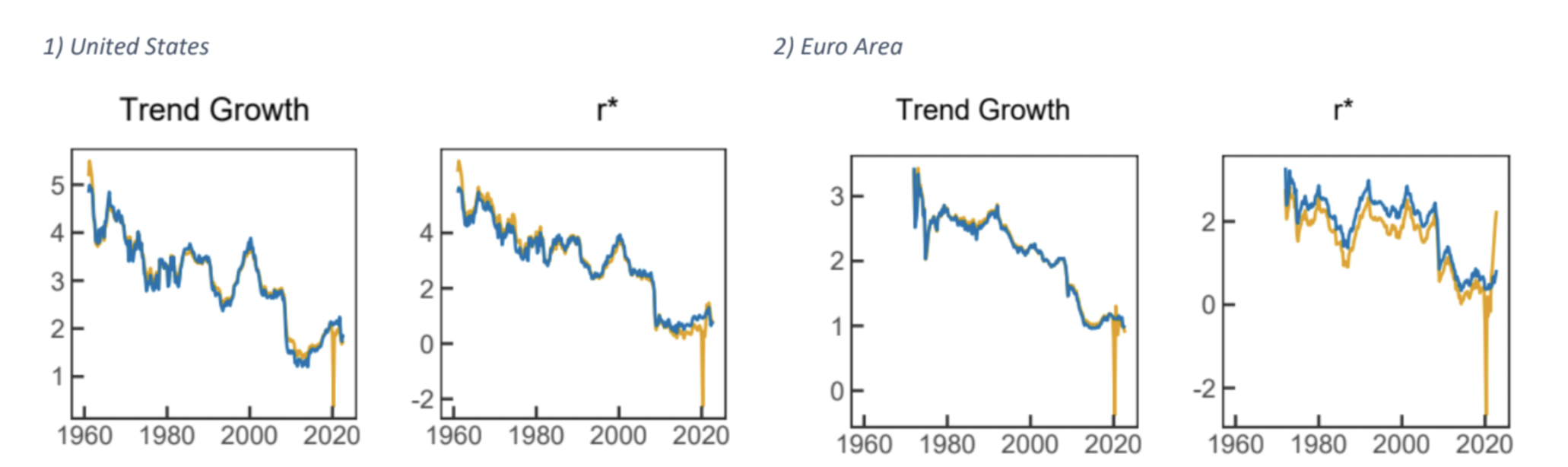
The blue line represents the COVID-adjusted model while the yellow line is the pre-adjustment one.
Source: Measuring the Natural Rate of Interest after COVID-19” – Holston, Laubach, Williams (2023)
The Effect of r* on Asset Class Returns
Having outlined what the main movements in r* are, we now move one to a short statistical analysis of the effect that this variable has had on returns, a topic on which there has not been much empirical research. Our prior belief as to why r* might have an impact on asset classes might not be completely apparent at first glance: We believe that current r* estimates might play a role in the expected return of those asset classes that are most directly related to long term economic growth.
Nevertheless, we test whether there is a statistical relationship between r* and various different asset classes. For this, we gathered quarterly r* estimates from the website of the New York Federal Reserve (using the updated HLW methodology) and quarterly asset class returns from Bloomberg. We use quarterly data because a higher frequency estimate of r* was not available. The specific assets/asset classes we compile return data for are the following: S&P500, NASDAQ, Gold, WTI Oil, Copper, US Treasuries, US IG Credit, US HY Credit. Lastly, we gather data for the risk-free rate from Kenneth R. French’s Website. Our data goes back to the first quarter of 1961 or some years later for time series that do not go back to 1961. With this assortment of asset classes, we believe to have represented a large portion of the investment opportunity set of an ordinary investor.
We then estimate the coefficients of a univariate OLS regression with the independent variable being r* and the dependent variable being returns or (in the case of the stock market indices) excess returns over the risk-free rate.
We get statistically significant loadings on r* for US Treasuries at the 5% level and for the S&P500 and NASDAQ at the 10% level; it should be mentioned that the R2 for all regressions is low at only a couple of percentage points. Returns for US Treasuries have a positive loading on r* while the two stock market indices have negative loadings. These findings are mostly in line with our ex-ante belief. Firstly, those asset classes that, in general, have the highest dependency on the general economy seem to have a statistically significant relationship to r* and secondly, the sign of the loadings make sense. For equities, a higher r* can be seen as a higher expectation for long-term interest rates, therefore decreasing the value of cash flows of future years and leading to negative returns. Since US Treasuries generally have a negative correlation to equities, a higher r* forecast leads to higher returns in Treasuries.
The Effect of r* on Factor Returns
Looking at the picture in equities, we were not fully content with finding a general relationship; therefore, we hypothesized that the same relationship that held true for equities in general can be applied to equities with specific characteristics. That is, equities with a higher dependency on the long-term growth of the economy will also have a relationship to r* estimates. In order to test this hypothesis, we used factor data downloaded from jkpfactors.com, a website giving access to many different factors and factor themes which was made in the course of the creation of Jensen, Kelly, Pedersen (2023), a paper that was already discussed in this BSIC article.
More specifically, we test all available themes for relationships. Namely, these are: Accruals*, Debt Issuance*, Investment*, Leverage*, Low Risk, Momentum, Profit Growth, Profitability, Seasonality, Size*, Skewness, Value. Those themes marked with a star (*) are themes in which one is short equities with high values for a characteristic and long equities with low values for a characteristic.
Running the same regression as before (we do not use excess returns for these factor themes), we get the following results:
Accruals, Debt Issuance, Profit Growth, Seasonality, and Skewness all are statistically significant at the 5% level. Keeping the above in mind, a higher r* is positive for portfolios that are either short in high accrual, debt issuance, and skewness equities and long low values for the respective characteristics, or long in high profit growth and seasonal equities and short in low values for these characteristics.
Once again, these results are easily reconciled with our prior expectation. Not only are equities with extreme values for these characteristics more strongly related to long term economic growth, but also does the sign of the loading make intuitive sense. To give an example, those companies that have a high seasonality are more susceptible to changes in long-term growth and if an economy can be sustained at a higher interest rate, then the economy shows more growth potential.
Conclusion
In this article, we have shown what the significance of r* is for economics and how it is estimated. As a financial application of r*, we have hypothesized that returns of assets that are more closely related to long-term economic growth will show a concurrent statistical relationship to r*. This intuition was proven correct in both asset classes in general and different factors specifically. However, more research will be needed in order to unravel the true underlying economic effects of r* on different asset classes and factors. Equally, a higher frequency estimate of r* could be used to more accurately review the statistical relationships we have found in this article.
Footnotes
1: Lewis and Vazquez Grande (2017); Buncic (2021); and Davis, Zalla, Rocha, and Hirt (2023) all argue in the direction of a higher r*
2: Also refer to “Measuring the Natural Rate of Interest after COVID-19” – Holston, Laubach, Williams (2023).
3: This opposite thesis is supported by the recent paper “R-star is higher. Here’s why” by Davis, Zalla, Rocha, and Hirt (2023). In this paper, the authors do not only claim that r* is now historically high but also that the era of secularly low rates is already over and a new era of “sound money” has begun.
References
[1] Laubach, T., Williams J.C., “Measuring the Natural Rate of Interest”, 2003, The Review of Economics and Statistics
[2] Holston, K., Laubach, T., Williams J.C., “Measuring the natural rate of interest: International trends and determinants”, 2017, Journal of International Economics
[3] Hale, T., et al., “A global panel database of pandemic policies”, 2021, Nature
[4] Lewis, K., Vazquez-Grande, F., “Measuring the natural rate of interest: A note on transitory shocks”, 2017, Journal of Applied Econometrics
[5] Buncic, D., “Econometric Issues with Laubach and Williams’ Estimates of the Natural Rate of Interest”, 2021, Available on SSRN
[6] Davis J.H., et al., “R-Star is Higher. Here’s Why”, 2023, Available on SSRN
[7] Holston, K., Laubach, T., Williams J.C., “Measuring the Natural Rate of Interest After COVID-19”, 2023, Federal Reserve Bank of New York
[8] Jensen, T.I., Kelly B., Pedersen, L.H., “Is There a Replication Crisis in Finance?”, 2023, Journal of Finance
TAGS: r-star, natural rate of interest, neutral rate of interest, factors, real rate


0 Comments