Introduction
Starting in 1992, a field of financial economics research emerged that has spewed out hundreds of so-called factors that help explain the “cross-section of expected returns”. Harvey and Liu (2019) [6] provide a taxonomy of some 400 different factors which they classify into 6 so-called “common” classes to which all assets have some level of exposure and 5 “characteristics” classes to which only some assets have exposure. The “common” categories are financial, macro, microstructure, behavioral, accounting, and other while the “characteristics” categories are all of the above except for macro which is by definition “common”.
In recent years, researchers have become weary of the ever-increasing number of factors that exist in what some aptly call the “Factor Zoo”, citing that at least a portion of proposed factors are the result of data mining. While investigating this hypothesis may seem like a purely academic endeavour at first, in reality, it has implications for the real world. Not only is the exposure to factors an important benchmark and source of inspiration for fund managers but the segment of mutual funds and ETFs that track some factors is multiple trillion dollars large.
The question of whether most factors are data-mined has sparked quite a debate in the financial economics research community. In this article, we will compare two influential viewpoints on the question: Firstly, the interpretation that most factors are, in fact, data-mined as per Harvey, Liu, Zhu (2016) [7] KellKand the opposing view of Jensen, Kelly, Pedersen (2021) [9].
Research on Factor Models is not Reliable
There are strong incentives to only submit results that validate the hypotheses set out by researchers since academic journals rarely publish negative results. This means that one cannot know how many hypothesized factors have actually been tested but never saw the light of day. Furthermore, most researchers do not account for transaction costs which inflates the returns of investment strategies on paper. Lastly, it is known that researchers are not immune to making errors when testing a given hypothesis even though peer review can reduce the size and amount of errors (for more information, please refer to Menkveld et al. (2021) [11]). All of this points to the fact that at least a portion of factors are either redundant (i.e. do not add explanatory power in a model) or irrelevant (i.e. do not explain returns). These falsely identified factors could simply be spurious results with good intentions or plainly the consequence of p-hacking. This can also be seen by a simple graph showing the probability of not incurring a type-I error in a certain number of (presumed to be independent) hypotheses with p-values of 0.05, 0.025, 0.01.
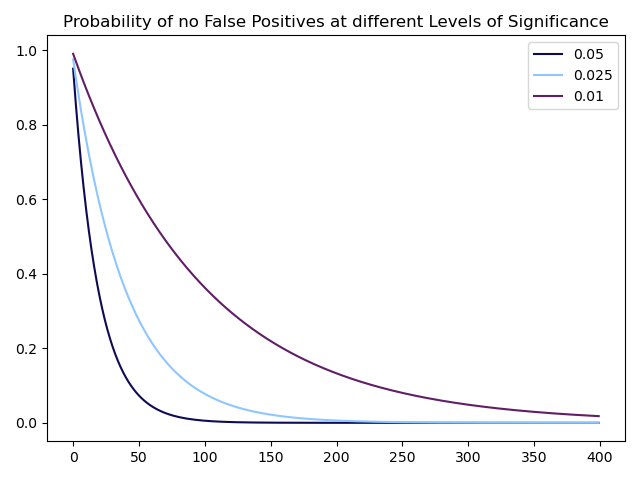
Source: Bocconi Students Investment Club
Put differently, this graph shows that if 400 discovered factors had a p-value of 5%, the chance that at least one of them is a spurious discovery is indistinguishable from 100%. The same is true if all factors had a p-value of 2.5% and even if they had a p-value of 1%, the chance of at least one spurious discovery is greater than 98%.
A simple fix for this problem would be decreasing the needed p-value to accept factors to a value such as 0.1%. In fact, some of the most well-known factors such as the Value or Momentum factors exhibit p-values below this threshold:
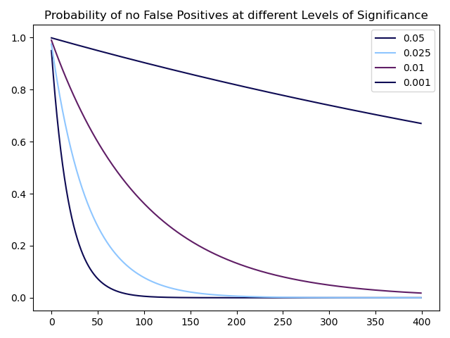
Source: Bocconi Students Investment Club
The caveat, however, is that the probability of a type-II error (not rejecting the null hypothesis even though it is false) rises with a decreasing p-value threshold, meaning many true factors would be rejected.
Nevertheless, Harvey, Liu, and Zhu propose different methods to obtain lower p-value/higher t-ratio thresholds that are adjusted for the fact that multiple hypotheses might have been tested in the discovery of potential factors. In general, two different approaches can be taken in order to infer new p-value thresholds: controlling for the so-called family-wise error rate (FWER) or for the false discovery rate (FDR). For a given level of significance and a number of discoveries, the FWER is defined as the probability of incurring at least one type-I error while the FDR is defined as the expected proportion of type-I errors in the discoveries. While the FWER could be considered the more natural approach to our problem, as can be seen above, it is extremely restrictive when the number of discoveries is large. In fact, a certain number of false discoveries may be tolerated as long as they do not exceed a certain proportion of the overall number of discoveries; something which is captured by the FDR.
More specifically, the authors use three different methods for adjusting the p-value thresholds: the Bonferroni and Holm adjustments both control FWER while the Benjamini, Hochberg, Yekutieli (BHY) adjustment controls FDR.
The Bonferroni adjustment is simple. For a given number of tests ![]() , it adjusts the original p-value threshold
, it adjusts the original p-value threshold ![]() downwards by a factor of
downwards by a factor of  , i.e. any hypothesis with a p-value
  is rejected. Therefore, the adjusted p-value of a given hypothesis test
  must be greater by a factor
  , as long as it is smaller than 1:

The Holm adjustment is more complicated in that it requires two steps. First, one orders the p-values of all hypotheses in increasing order such that  of the associated null hypotheses
  . Second, one defines
  as the smallest index for which it holds
  for a given p-value threshold
  . Then one rejects only the null hypotheses
  . The adjusted p-value of a given hypothesis test
 ![]() now is:
now is:
![]()
This adjustment is more lenient towards rejections of the null hypothesis (i.e. the discovery of factors) than the Bonferroni adjustment in that those factors discovered using the Bonferroni adjustment form a subset of those discovered using the Holm adjustment.
Lastly, the BHY adjustment follows a two-step procedure: First, one orders the p-values of all hypotheses in increasing order such that of the associated null hypotheses . Second, one defines ![]() as the largest index for which
as the largest index for which  holds for a given p-value threshold
  and
and  . One then rejects all null hypotheses
  and the corresponding p-value for a given hypothesis test is:

Using these three adjustments, the authors then derive a lower bound of the necessary p-value thresholds that account for multiple testing. The thresholds are lower bounds because of the (knowingly false) assumption that the number of discovered factors is equal to the number of tested factors. The original threshold chosen by the authors for the first two adjustments is  while the BHY adjustment calls for a lower original threshold of
  since the FDR is a weaker control than the FWER.
The results are the following: For 316 proposed factors, the newly adjusted p-value thresholds for the Bonferroni, Holm and BHY adjustments are 0.02%, 0.01%, and 0.07% respectively. For the first two methods, the adjusted p-value thresholds will continue to decrease with a larger number of proposed factors; however, as explained above, controlling for the also FWER becomes less sound with more tests. Meanwhile, the adjusted threshold for the BHY adjustment converges towards one value.
Taking into account further considerations, the authors conclude that a t-ratio threshold of 3.0 which corresponds to a p-value of 0.27% should be used as a threshold for future factor research but concede that even such a threshold might be too low. In fact, other research such as Chordia et al. (2020) [2] has concluded that t-statistics of 3.4 to 3.8 (p-values of 0.07% to 0.015%) are necessary. Lastly, while out of the scope of this article, the use of machine learning in order to discover false positives has seen some use; the interested reader should refer to de Prado and Lewis (2019) [3] and Giglio et al. (2021) [5].
Economic Research on Factor Models
Factor investing has been widely studied, but confusion and myths persist, especially after the 2018-2020 underperformance of multi-factor portfolios. As already mentioned, one of the most often cited critiques of factor research is that factors are data-mined, due to the over-examination of financial data. This is an absolutely valid concern, as financial literature has been flooded with a host of factors claiming to predict returns, which is quite unexpected, considering the overall efficiency of markets. Because of that, there is a need for a coherent economic explanation behind them.
The main idea behind factor investing is that there are more dimensions to building efficient portfolios than simply taking on market risk, Merton (1973) [10], and Ross (1976) [12]. Factors can deliver positive returns beyond market risk, either due to compensation for additional risk exposure or because they exploit or counter different preferences or beliefs among investors. Thus, we could divide economic factor research into risk-based and behavioral. Risk-based factors provide risk premia or sources of positive expected returns, while behavioral factors focus on preferences or beliefs that deviate from classic wealth-maximizing objectives (Fama and French (2015) [4], Shleifer (2000) [13], Thaler (2003) [14], Barberis (2018) [1]). However, understanding the source of returns and why they persist requires examining why they do not get arbitraged away and identifying who/why are the investors willing to take the other side of these factor trades (Ilmanen et al., 2022) [8]. For the sake of simplicity, we would only focus on the four most prominent factors in the financial literature: value, momentum, carry, and defensive/quality.
Value investing involves buying undervalued stocks and is typically measured by ratios such as price-to-book, price-to-earnings, or price-to-cash. Risk-based explanations for the value premium argue that value stocks are riskier, as they often represent distressed companies or industries, while behavioral ones suggest that investors may overreact to negative news or have biased expectations, leading to an undervaluation. Momentum investing seeks to capitalize on recent stock performance by purchasing stocks that have outperformed and selling those that have underperformed. The momentum premium is thought to compensate for risk, especially for stocks sensitive to changing economic conditions, and behavioral explanations attribute it to things like “herding”, underreacting to news, and anchoring biases. A carry trade on the other hand involves borrowing at a low-interest rate and investing in an asset providing a higher rate of return or simply buying high-yielding assets while selling low-yielding ones. Carry returns usually represent compensation for risk, particularly in times of financial stress or liquidity constraints, but some behavioral explanations propose that investors may be biased towards high-yielding assets, leading to excessive demand and higher prices. Defensive/Quality investing emphasizes low-volatility, low-beta, and high-quality stocks, assessed by factors like profitability, stable cash flows, and financial strength. These stocks offer lower but more stable returns due to their low credit risk. Nevertheless, behavioral factors may cause investors to be attracted to high-volatility stocks, resulting in overpricing and underperformance.

Source: Portfolio Management Research
In summary, factor investment strategies are not simple arbitrage opportunities Each of these factors is driven by a combination of risk-based and behavioral explanations. The precise reasons for their persistence may differ, but they generally involve a mix of risk compensation and the exploitation of investors’ biases or preferences. They offer long-term positive expected returns but can also experience poor performance from time to time. Risk-based explanations for these factors emphasize that eventually risks do materialize and are most of the time unavoidable, thus justifying the premium. Experiencing these risks can be unpleasant, but they ultimately imply a premium over time. Undiversifiable drawdowns or those occurring at the most painful times determine who is on the other side of each factor strategy. Investors who cannot tolerate short-term fluctuations may forgo the long-term expected return premium to avoid risks. In this sense, factors can be seen as insurance or hedging portfolios, allowing risk-averse investors to pay a small premium to those willing to bear the risks. This creates a natural equilibrium where factors earn long-term returns due to supply and demand for risk-bearing.
Behavioral explanations also provide a natural set of investors on the other side of factor trades. For value, growth trend-chasing investors are willing to pay higher prices for the latest growth and tech firms, while momentum, carry, and defensive strategies each have their own sets of investors with specific preferences and risk tolerances. These explanations are not mutually exclusive, and a premium associated with a factor can be driven by both risk and behavioral forces. Both sets of theories offer a solid economic rationale for why a premium exists and is expected to persist, often with testable or observable implications beyond returns. The changing risk appetite, preferences, and beliefs of investors over time can lead to variations in the size of these premiums.
Statistical and Out of Sample Testing
Of course, there are other ways to evaluate the validity of factors like testing on out-of-sample data and performing formal statistical assessment. As already discussed a lot of research papers like Harvey, Liu, and Zhu (2016) [7], have pushed for more rigorous testing, advocating for higher statistical significance standards, and reducing the number of reliable factor discoveries. Despite this, factors such as value, momentum, carry, and defensive/quality still pass these stringent tests, indicating that critics are not rejecting factors altogether but seeking a more rigorous selection process for determining the factors that truly matter.
Since errors are random, research that overfits errors through data mining in the original sample should fail to produce significant results when applied to a separate, independent sample. Various methods can be employed to obtain out-of-sample evidence, such as examining different time periods within the original sample, exploring markets that were not initially investigated, or considering alternative asset classes.
Ilmanen et al. (2021) for example conducts a thorough analysis of the out-of-sample performance of primary factors, including value, momentum, carry, and defensive/quality. The study spans a century of data across multiple markets and asset classes, such as US stocks, global stocks, equity indices, currencies, fixed income, and commodities. By examining both pre-sample and post-sample evidence, the research demonstrates the stability and efficacy of these factors across different periods and markets and reveals that they perform consistently across almost all markets and asset classes, with stable performance in both pre and post sample periods. Notably, there is robust evidence of factor returns prior to the original samples, suggesting that these factors generated significant returns before researchers even began studying or conceptualizing them. The similar performance in the post-sample period (after the discovery of the factor investing) further indicates that these strategies are not merely a result of data mining and are unlikely to have been arbitraged away. While their factors are not optimized and can be enhanced through diversification across different measures of the same phenomenon and other design choices that improve implementation efficacy, they offer simple, replicable factor series that effectively capture the premia.
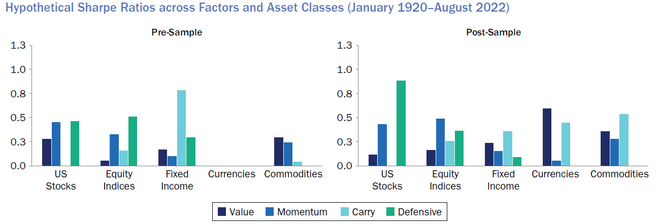
Source: Portfolio Management Research
In another recent paper titled “Is There a Replication Crisis in Finance?”, Jensen, Kelly, and Pedersen (2021) [9] question whether there truly is a replication issue in the field of finance. The authors argue that the supposed large number of factors that some papers cite (400+) is significantly exaggerated, as most of these factors are just different versions of the same theme. For instance, over 80 versions of value signals like book-to-price ratio vs. earnings-to-price ratio, are all highly correlated, as well as there are numerous measures of momentum. These should not be considered independent factors, instead, the authors propose a factor taxonomy that algorithmically classifies factors into themes, characterized by a high degree of within-theme return correlation and similarity of economic concept. To test their hypothesis, they employ a Bayesian framework to evaluate the out-of-sample performance of these factors and argue that a prior of zero alpha, which is reasonable if markets are efficient, would lead to expectations of lower out-of-sample performance, as returns should shrink towards that prior, given that the truth is a combination of theory (e.g., one’s prior) and data (measured with error). This implies that positive but lower out-of-sample performance should be expected and not necessarily viewed as evidence of overfitting. Furthermore, the paper examines the factors together, combined into one portfolio, considering that factors provide diversification benefits. The performance of the tangency portfolio of fares even better out-of-sample, as diversification across factors mitigates noise in each individual factor.
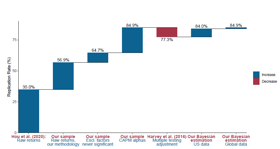
Source: Jensen, Kelly, and Pedersen (2021)
Conclusion
Addressing data mining concerns is essential for instilling confidence in factor-based strategies. This can be achieved by seeking strong theoretical foundations and robust out-of-sample evidence. Despite the possibility of some false positives, the overwhelming statistical and economic evidence supporting the existence and significance of factors is hard to dismiss. Continuous research in understanding existing factors is as crucial as discovering new ones, as it can lead to better performance, increased confidence during drawdowns, and the ability to identify regime changes. Focusing on out-of-sample evidence, refining factor measurement, and enhancing understanding of known factors can contribute to a more resilient investment approach. Ultimately, ongoing research in known factors, backed by substantial evidence, can be invaluable in maximizing their benefits, improving performance, and adapting to changing market conditions.
References
[1] Barberis, N. 2018. “Psychology-Based Models of Asset Prices and Trading Volume.”
[2] Chordia et al., 2020, “Anomalies and False Rejections”
[3] de Prado and Lewis, 2019, “Detection of false investment strategies using unsupervised learning methods”
[4] Fama, E. F., and K. R. French. 2015. “A Five-Factor Asset Pricing Model.” Journal of Financial Economics
[5] Giglio et al., 2021, “Thousands of Alpha Tests”
[6] Harvey and Liu, 2019, “A Census of the Factor Zoo”
[7] Harvey et al., 2016, “… and the Cross-Section of Expected Returns”
[8] Ilmanen, A., R. Israel, R. Lee, T. J. Moskowitz, and A. Thapar. 2021. “How Do Factor Premia Vary over Time? A Century of Evidence.” Journal of Investment Management
[9] Jensen et al., 2021, “Is There a Replication Crisis in Finance?”
[10] Merton, R. C. 1973. “An Intertemporal Capital Asset Pricing Model.
[11] Menkveld et al., 2021, “Non-Standard Errors”
[12] Ross, S. A. 1976. “The Arbitrage Theory of Capital Asset Pricing.” Journal of Economic Theory
[13] Shleifer, A. Inefficient Markets: An Introduction to Behavioural Finance. Oxford University Press UK. 2000.
[14] Thaler, R., and N. Barberis. “A Survey Of Behavioral Finance.” Handbook of the Economics of Finance. Elsevier. 2003


0 Comments