Catching the Butterfly: A Relative Value Approach in OIS Curves

Introduction

Principal component analysis is widely used for explaining and hedging in the interest rates markets due to its construction based on orthogonality which pairs well with the multicollinearity prevalent in rates. Its explanatory power is able to consistently explain over 95% of the variance in yield curve movements through its first 3 principal components. For this reason, we can construct theoretical fair value yield curves that, when overlapped on the actual yield curves, can provide trading signals showing local dislocations.

In this article we will first explain the methodology behind a fair value curve reconstruction applying it on three different OIS curves, we later present the reasons and approach to test for mean reversion and apply that notion on a series of forward strips to capture the forward starting nature of the trade. We end by pitching the best ranked trade on an adjusted scoring system and reconnect the model’s reasoning with the macroeconomic perspective subtended in the trade pitch.

Explaining the PCA Method (First 3 PCs, Math etc.)

Using PCA we can reconstruct theoretical swap curves and then compare them to the actual current swap curve to assess the extent to which swap rates deviate from their theoretical fair value. PCA is a powerful statistical tool that works best on a highly colinear system such as interest rate term structures. We use PCA to extract the key sources of variation from the data, thus simplifying the representation of yield curve dynamics.

We applied this methodology to USD SOFR, EUR €STR, and GBP SONIA curves as a framework of identifying relative value opportunities across those curves.

A swap curve is a vector $r_t \in \mathbb{R}^N$ of $N$ rates at fixed maturities (here $N = 15$ tenors from 1y to 30y) observed daily. This vector is highly colinear as for most days, rates move in the same direction by roughly the same amount, which is why the $N$ -dimensional series sits inside a much lower-dimensional subspace. PCA rotates this basis of $\mathbb{R}^N$ to one in which the new coordinates are uncorrelated and ordered by variance.

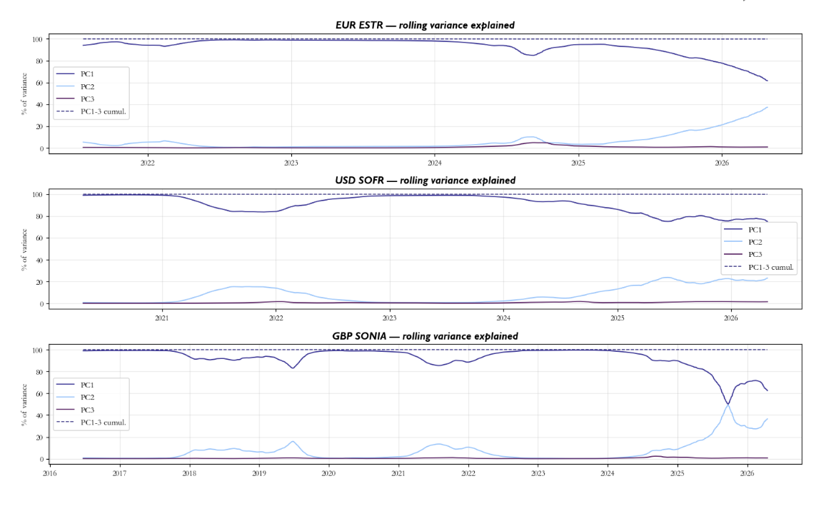
In rates the empirical observation is that the first three principle components (PCs) explain well over 95% of the variance of any developed market swap curve which we were able to confirm within our data.

We start our PCA analysis by defining our setup with $r_t = (r_{t,\tau_1}, \dots, r_{t,\tau_N})^\top$ being the curve on day $t$ , where $\tau_j$ are the tenors. We picked a common rolling window of 1 years ( $W = 261$ business days) and we take the $W \times N$ matrix of rate levels over the window, subtract the cross-sectional time-series mean from each tenor column, and form:

$\bar r = \frac{1}{W} \sum_{s=t-W+1}^{t} r_s, \qquad X = \begin{bmatrix} (r_{t-W+1} - \bar r)^\top \ \vdots \ (r_t - \bar r)^\top \end{bmatrix} \in \mathbb{R}^{W \times N}.$

The sample covariance matrix is

$\Sigma = \frac{1}{W-1} X^\top X \in \mathbb{R}^{N \times N}.$

This is the covariance of mean-centred rate levels as the goal of the first-stage PCA is to reconstruct where rates sit on the curve, not how much they move day to day. Working on levels captures the factor structure of the curve’s shape over time, which is exactly what is needed to define a fair-value level for each tenor.

Because $\Sigma$ is symmetric and positive semi-definite, the spectral theorem gives

$\Sigma = L \Lambda L^\top,$

with $\Lambda = \mathrm{diag}(\lambda_1, \dots, \lambda_N)$ , $\lambda_1 \ge \lambda_2 \ge \dots \ge \lambda_N \ge 0$ , and $L$ orthogonal. The columns $L_{\cdot k}$ are the PCA loading vectors (eigenvectors of $\Sigma$ ); $\lambda_k$ are the eigenvalues, and the fraction of variance explained by component $k$ is $\lambda_k / \sum_i \lambda_i$ .

For any rate vector $r_t$ , the scores are the projections onto the loadings:

$y_{t,k} = L_{\cdot k}^\top (r_t - \bar r), \qquad k = 1, \dots, N.$

Because $L L^\top = I$ , the original rates are recovered exactly by

$r_t = \bar r + \sum_{k=1}^{N} y_{t,k} , L_{\cdot k}.$

If we only keep the first three components, we get the PCA fair value:

$\hat r_t = \bar r + \sum_{k=1}^{3} y_{t,k} , L_{\cdot k}.$

The residual surface is

$\varepsilon_t = r_t - \hat r_t = \sum_{k=4}^{N} y_{t,k} , L_{\cdot k}.$

Intuitively, this means that we project the swap curve onto the 3D subspace spanned by the first three PCs and treat the residuals as noise or a tradable dislocation.

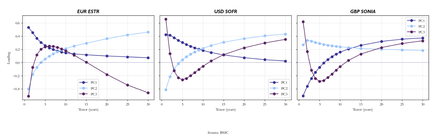
The first three PCs in our case, and in general for interest rate term structures, represent parallel shifts, changes in slope and changes in convexity of the curve. In perfectly correlated system of changes in interest rates or levels in interest rates, the factor loadings of the first PC would be equal. More generally, the more correlated the system, the more similar the values of the loadings of the first PC across the variables. As such, the first PC captures a common trend in the variables. So, if the first PC changes and the other components remain fixed, then the variables in your system, in this case the interest rates, will all move by roughly the same amount. Thus, we consider PC1 as a measure of the level of yields.

The loadings of the second PC typically decrease (or increase) in magnitude with maturity. As such, if PC2 changes while the other components remain the same, then the rates at one end of the term structure will move up and the others will move down. For this reason, PC2 can be considered a proxy to the slope of the curve.

Similarly for PC3, the loadings of PC3 typically decrease (or increase) in magnitude and then increase (or decrease). As such, if PC3 changes while the other components remain constant, then the rates at either end of the term structure will move up, and the rates in the middle will move down. In the graph shown previously you can see how the explained variance by the respective PC changes over time while below we show how the factor composition of the respective swap curve evolves.

Findings

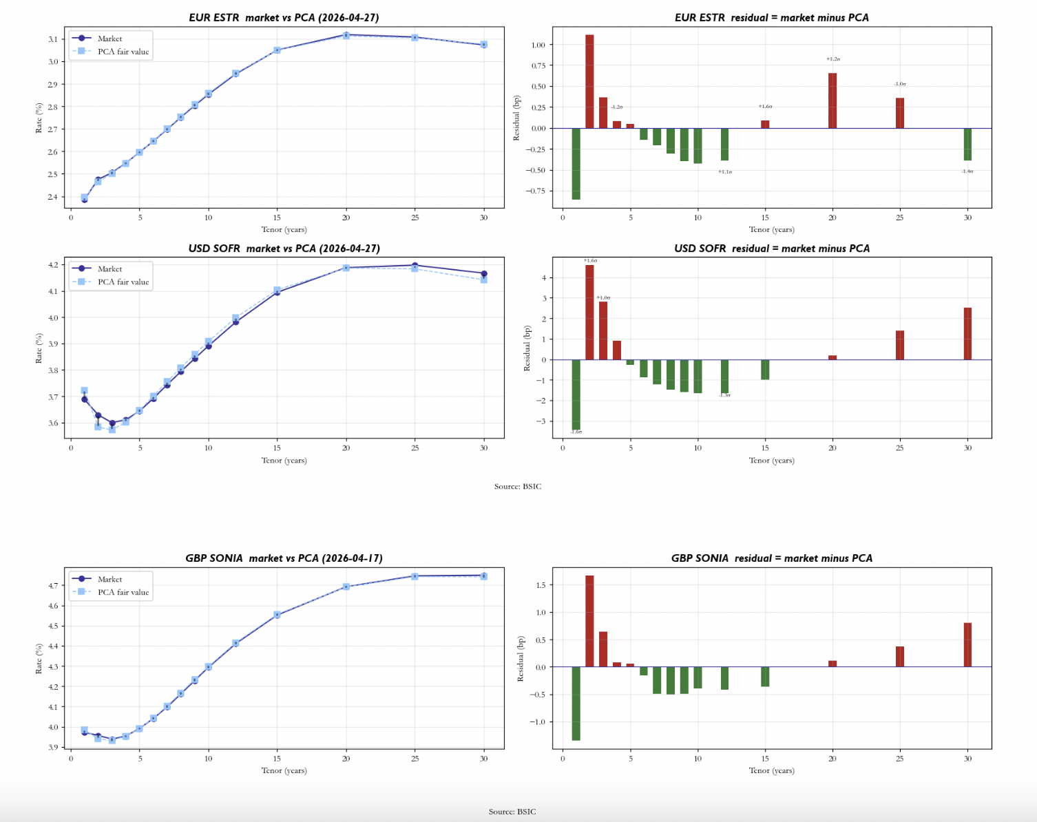
Now that we have laid out our methodology, we can decompose the respective swap curves and reconstruct them using the first three PCs for each. After decomposing them, we reconstruct the theoretical fair value curve using only the first three PCs and then compare it with the actual swap curve, identifying tenors on the curve that might be mispriced or rather as a discretionary relative value tool that helps you inspect that helps you choose the best structure on expressing a directional trade that you plan to put on. Below we show our PCA’s most recent comparison of the theoretical against the actual swap curve.

After building our residual curve, we scan for potential trades by identifying combinations of tenors where the PCA-flagged dislocations align in the right pattern and then testing whether those combinations have historically corrected themselves.

The residual surface gives us a Z-score for every tenor at every date. For a butterfly, the sign filter requires that the two wings sit on the same side of fair value while the belly sits on the opposite side. For a curve trade, we simply require that the two legs have opposite-signed Z-scores: one rich, one cheap. This sign filter is the first gate. Most of the candidate list, eleven butterfly templates and twelve curve templates per currency, is eliminated here on any given day, because the residual surface rarely has the sign pattern required. What passes through is a small set of structures where the curve genuinely appears dislocated in a tradable configuration.

For each surviving candidate we construct two time series going back through the full history of available data (have to add the time here). The actual spread $S_t$ is the PCA-neutral combination of the raw market rates.

$S_t = c_1 , r_{t,\tau_1} - r_{t,\tau_2} + c_3 , r_{t,\tau_3} \quad \text{(butterfly)}$

The fair-value spread $\hat{S}_t$ is the identical combination applied to the PCA-reconstructed curve rather than the market curve:

$\hat{S}t = c_1 , \hat{r}{t,\tau_1} - \hat{r}{t,\tau_2} + c_3 , \hat{r}{t,\tau_3}$

The trade dislocation is their difference, converted to basis points:

$D_t = 100 \cdot (S_t - \hat{S}_t)$

This is the object everything else is run on. The key insight is that $D_t$ measures how far the trade itself sits from where PCA thinks it should be, not how far any individual rate sits from fair value. Individual tenor residuals can move around for all sorts of reasons. The question we actually care about is whether the spread that packages those residuals into a tradable structure has a memory and pulls back to zero.

The Augmented Dickey-Fuller Test

The first question we ask of $D_t$ is whether it is stationary at all. A non-stationary series has no well-defined mean to revert to, so the entire mean-reversion narrative collapses. We test this with the Augmented Dickey-Fuller (ADF) regression:

$\Delta D_t = \alpha + \beta , D_{t-1} + \sum_{i=1}^{p} \gamma_i , \Delta D_{t-i} + \varepsilon_t$

The lagged level term $\beta D_{t-1}$ is the heart of the test. Under the null hypothesis $H_0: \beta = 0$ , the series has a unit root, meaning that it drifts without bound and has no tendency to return to any level. Under the alternative $H_1: \beta < 0$ , the lagged level pulls the series back toward its mean. The lags $\Delta D_{t-i}$ are included to absorb any serial correlation in the residuals that would otherwise bias the test and the number of lags $p$ is chosen automatically by minimising the Akaike Information Criterion.

The ADF is run on a trailing window of 1 year (261 business days) of the dislocation series. This window is kept independently of the PCA window (2 years), as the PCA defines our fair-value curve over a full cycle, while the ADF asks whether mean reversion is present in the current regime. A potential trade passes our filter if the ADF $p$ -value is below 10%.

The AR(1) Half-Life

Passing the ADF test tells us that $D_t$ is stationary, but it says nothing about how quickly it reverts. For purposes of trade sizing and holding period decisions we fit a first-order autoregression (AR(1)) on the same ADF window lookback.

$D_t = \alpha + \rho , D_{t-1} + \eta_t, \qquad 0 < \rho < 1$

The constant $\alpha$ allows the dislocation to oscillate around a non-zero unconditional mean $\mu = \alpha/(1-\rho)$ , which is more realistic than forcing the process to be zero-mean. The slope $\rho$ is estimated by OLS regression of $D_t$ on $D_{t-1}$ with a free intercept. The half-life depends only on $\rho$ :

$\mathrm{HL} = \frac{\ln 2}{-\ln \rho}$

The derivation is straightforward as we start from a dislocation of size $D_0$ , the expected gap to the unconditional mean decays as $\rho^k$ after $k$ days. Setting $\rho^k = 1/2$ and solving for $k$ gives the formula above.

A potential trade only makes it onto the recommended list only if all three of the following hold simultaneously. The lifetime Z-score must exceed 1.0 in absolute value, meaning the spread is at least one standard deviation from its mean. The ADF p-value on the trade spread must be below 10%, and the fitted autoregression is actually mean reverting and not explosive.

Most candidates do not pass the ADF filter due to elevated macro uncertainty, a central bank that has not yet anchored terminal rate expectations, or a structural curve shift. However, the trade can still be represented as the best instrument structure for an already existing directional view, but should also be framed as such and not statistical arbitrage.

Why forwards?

The framework laid out so far identifies dislocations on the swap curve and packages them directly into a PCA-neutral curve and butterfly spreads. This process however presents some ambiguity in the spot signal. Take for example the 5y point on the spot curve, if the model flags the 5y as cheap, whether the cheapness reflects an overshoot in the imminent policy path or a mispricing of the 4y1y forward rate is unknown. This is due to the fact that a single zero rate at maturity T is, by construction, the weighted average of every instantaneous forward between today and T.

Since the latest part of this article will attempt pitching a trade idea, without addressing a grid of forward starting OIS we would end up implementing a trade which is necessarily a forward-starting structure. Therefore, for the remaining part of this article, we will implement the entire pipeline: fair value reconstruction, residual z-scoring, sign filter candidate selection and PCA neutral weighting on a grid of forward starting par OIS rates.

To construct the forward curves, we define nine forward starts (spot, 1m, 3m, 6m, 1y, 2y, 5y, 7y, 10y) crossed with thirteen swap tenors (1y through 30y, including 4y and intermediate points). For each date and each (forward start, swap tenor) pair we need a par rate. Let z(T) denote the BoE continuously-compounded zero rate at maturity T years. The discount factor at maturity T is then: $D(T) = \exp(-z(T) \cdot T)$ .

A standard OIS pays a single fixed coupon (annual frequency for GBP) against compounded overnight SONIA. The float leg present-value is approximately D(T1) − D(T2) where T1 is the forward start and T2 is the maturity. The fixed leg present-value is the par rate K times the annuity, where the annuity is the sum of day-count fractions weighted by intermediate discount factors: $K_{par} = \frac{D(T_1) - D(T_2)}{\sum_{i} \alpha_i \cdot D(t_i)}$ .

We use Act/365 day counts (α ≈ 1.0 for annual periods) and a flat schedule running from T1 to T2 in one-year steps. Discount factors at non-grid maturities are obtained by linearly interpolating z(T) between BoE node maturities. Forwards whose terminal date T2 lies beyond the BoE maximum maturity are returned as missing rather than extrapolated.

Since the BoE already publishes a fitted spot curve, we observed that going via discount factors directly is more transparent, faster, and avoids a bootstrap step that can be fragile when input quotes are missing. The BoE smoother removes single-day microstructure outliers that would otherwise leak into our residuals.

This approach presents some weaknesses as OIS rates are smooth in the discount factor rather than in the (rate, T) plane. Log-linear interpolation of D(T) would give marginally tighter forwards starting between BoE nodes. The effect is sub-basis-point in normal markets, however during stressed or dislocated markets this can cause an amplification in forward distortions. Also, forwards with terminal date beyond the BoE maximum become missing. A Nelson-Siegel-Svensson or a flat-instantaneous-forward tail would let the dashboard cover 5y25y forward, and similar long-tenor combinations.

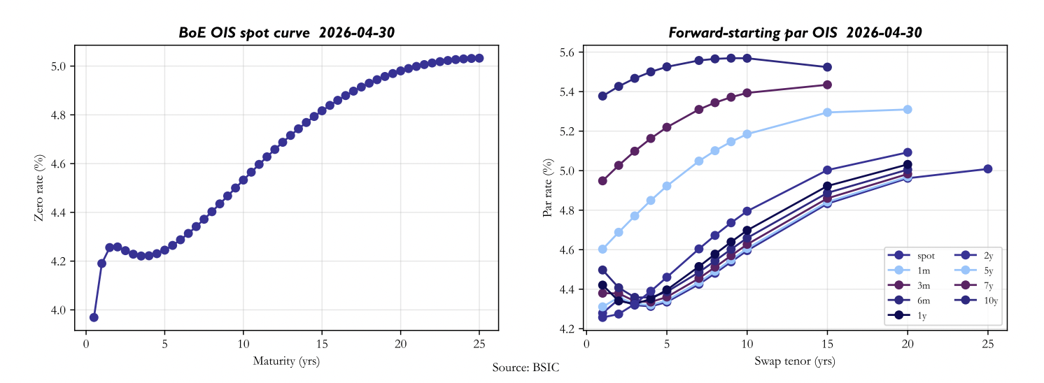
Spot through one-year forward strips capture the immediate policy path; two-year and five-year forwards strip out the policy cycle and isolate term-premium and growth expectations; the seven-year and ten-year forwards are dominated by long-end pension and insurance flows and tend to be smoother.

Across each forward strip we keep tenors from one year to thirty years. Thirteen tenors is enough to make the PCA meaningful and small enough that three components reliably explain more than ninety percent of the variance. The 4y, 8y, and 9y tenors are intentionally included even though they are slightly less liquid: they help the PCA fit the curvature region around the five-year and ten-year hump.

For each forward strip and each historical date we fit a three-component PCA on the previous 261 trading days (approximately one calendar year). The current day’s curve is then projected onto the principal components and reconstructed; the residual between the actual rate and the reconstruction is the cheap-rich signal. As previously mentioned, the first three components: PC1/2/3 should respectively be an indicator of level, slope, and curvature.

Just for expositions sake we show how the first 3 principal components, tested full sample, comove with related proxies.

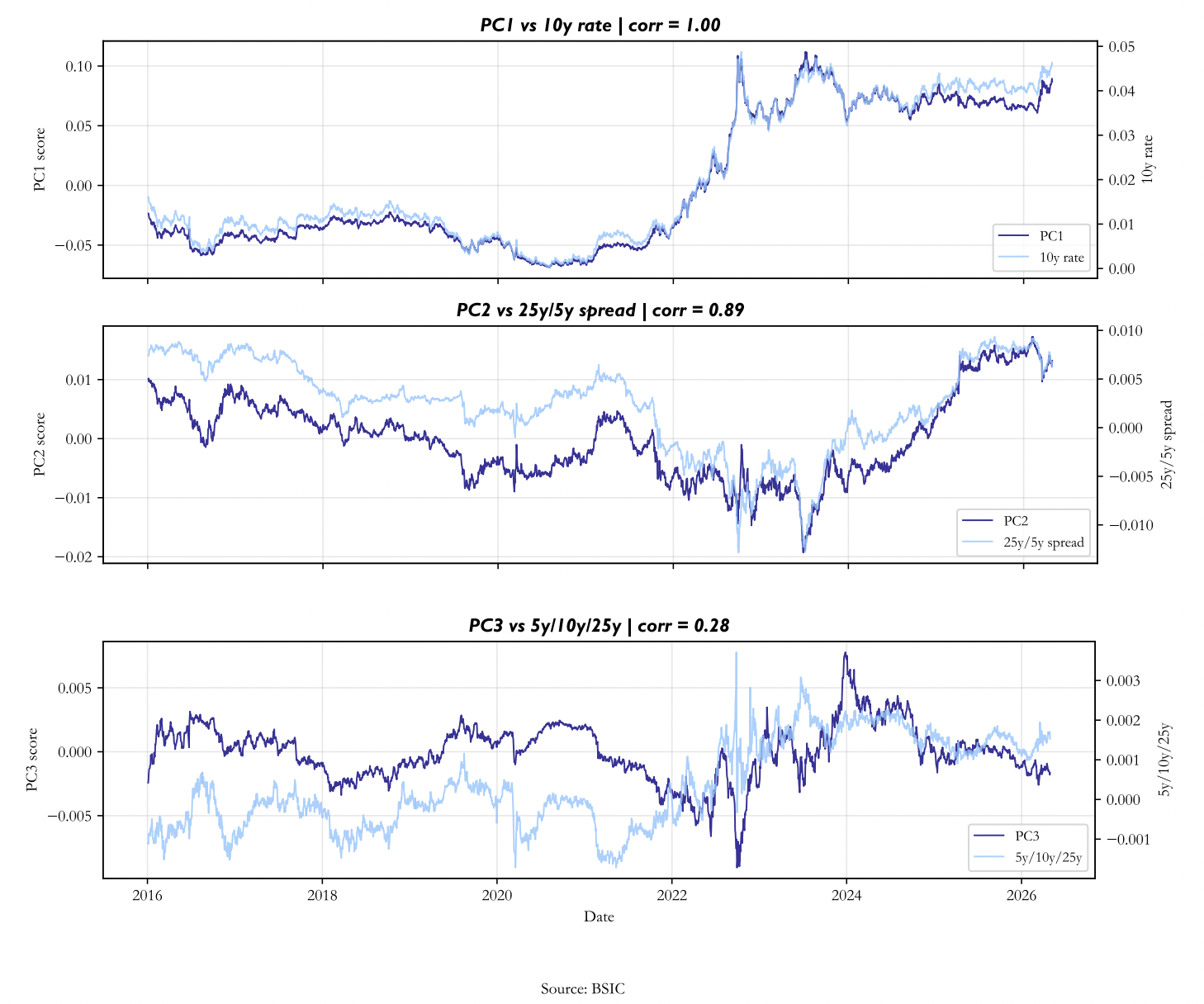We use a rolling fit rather than a full-sample fit for two reasons. First, the in-sample principal components contain forward-looking information that would invalidate any claim of an unbiased signal at the snapshot date. Second, the term-structure regime evolves: the level component in 2022 looked very different from 2025, and forcing the PCs to span both produces components that capture neither well. The choice of rolling window is highly discretionary, we chose 261 days as a proxy for a calendar year, shorter windows are more responsive but noisier; longer windows smooth out genuine regime change.

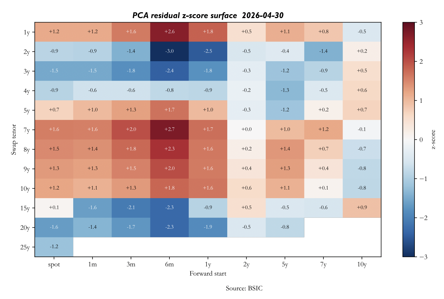
Once the residuals for each forward, tenor pairs are extracted, we can run the z-score, on the same window as the PCA, to understand the relative dislocation from the standardised average. A positive z indicates the rate is high relative to recent fair value (cheap to receive); a negative z indicates the rate is low (rich, pay).

Z-scores beyond ±2 are unusual in calm volatility regimes and beyond ±3 are rare. We use a minimum threshold of |z| = 1.0 to admit a tenor into the candidate trade pool. This deliberately wide net catches mild dislocations that, when combined into a PC-neutral curve or fly, can score well on the risk-adjusted ranking even though no single leg is strikingly extreme.

Trade Identification

For the trade identification we address two structures: two-leg curve trades, and three-leg butterfly trades.

The curve trades are identified by evaluating, through every forward strip, every rich tenor with cheap tenors and we admit only pairs in which the rich leg has a shorter tenor than the cheap leg. We chose this to maintain the trades economically meaningful and essentially only entering a flattener or steepener position rather than an arbitrary spread which might act like a butterfly fragment. Pairs are scored by the sum of the absolute z-scores across the two-legs.

Butterfly trades are identified initially by imposing at least one year of spacing between all triples of tenors (left,belly,right). The dislocation metric is: $\mathrm{dislocation} = \mathrm{belly}_z - \frac{\mathrm{left}_z + \mathrm{right}_z}{2}$ . A positive dislocation implies that the belly is cheap compared to the wings z-score, hence calling for a receive-belly/pay-wings position. A negative dislocation calls for the opposite. Candidates are ranked by absolute dislocation if they pass the minimum threshold of absolute dislocation score ≥ 1.0.

To determine ex-ante the attractiveness of the trade we take into consideration transaction costs. For each trade identified we adopt a deliberately simple bid-ask heuristic that widens with both swap tenor and forward start to reflect declining liquidity:

$\mathrm{bid\_ask\_bps}(t, f) = 0.25 + 0.05 \cdot \min(t, 30) + 0.04 \cdot \min(f, 10)$ .

where t is the swap tenor in years and f is the forward start in years. The constants are calibrated against on-screen IDB quotes for liquid GBP OIS in stable conditions. Per-leg costs are summed and weighted by the absolute notional of each leg, giving a round-trip cost in basis points of the trade level. This approximation clearly exposes some weaknesses; a simple improvement could be scaling the transaction costs based on an implied volatility proxy.

We approximate the one-day ex-ante roll-down under an unchanged curve by re-pricing each leg at a tenor one calendar day shorter, using linear interpolation of the rate over maturity on the snapshot day’s curve. The signed sum across legs, scaled by trade weights and direction, gives a basis-point estimate of how much the trade earns if the curve does not move overnight. True OIS carry from t to t+1 also includes the daily SONIA fixing differential against the accrued fixed coupon, however short horizons and on a flat or gently upward-sloping curve this is small and a rough estimation could be materially unprecise.

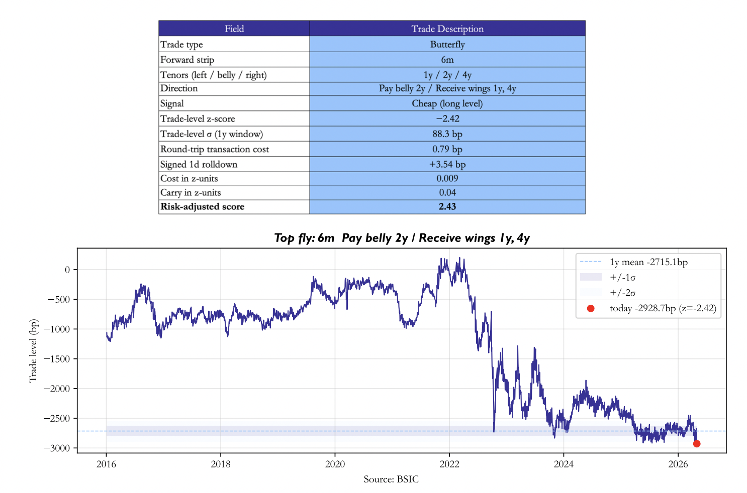
To evaluate each candidate on a single comparable scale we define an adjusted score. We define the PCA weighted sum of the leg rates over time and compute its rolling one year mean and standard deviation. The trade-level z-score is then a more honest summary than summing leg z-scores, because it uses the trade’s own residual volatility rather than the volatility of its underlying tenors. Cost and carry are converted to z-units by dividing by the same trailing standard deviation, in basis points:

$\mathrm{score} = \left|\mathrm{level}_z\right| - \mathrm{cost}_z + \lambda \cdot \mathrm{carry}_{z,\mathrm{signed}}$

$\mathrm{cost}_z = \frac{\mathrm{round\_trip\_cost\_bps}}{\sigma_{\mathrm{level\_bps}}}$
$\mathrm{carry}_{z,\mathrm{signed}} = \mathrm{position\_dir} \cdot \frac{\mathrm{rolldown\_bps}}{\sigma_{\mathrm{level\_bps}}}$
$\mathrm{position\_dir} = -\mathrm{sign}(\mathrm{level}_z)$

The default λ is 0.5, giving carry roughly half the weight of the entry-edge net of cost. Increasing λ biases the screen toward trades that pay you to wait; decreasing it biases it toward larger pure dislocations.

The dashboard ranks all candidates by score and presents the top trade in each category. The dashboard’s top-ranked candidate on the 30 April 2026 snapshot is a butterfly on the 6m forward strip, paying (fixed) the 2y belly against receiving (fixed) the 1y and 4y wings.

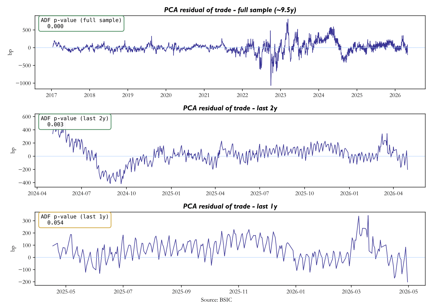
This entire approach using PCA z-score presupposes mean-reversion, hence before recommending this trade we test whether the residual time-series is stationary using the Augmented Dickey Fuller Test. We test for stationarity on three different windows. On the ten-year window, the ADF test yields a pvalue of ≈ 0.00. Restricting the mean-reversion test over the most recent 2-year window gives a p=0.003, providing a strong rejection of the unit root and evidence of the residuals mean-reversion tendency. The borderline p-value of 0.054 appears only on the trailing one-year window and is best read as a small-sample power limitation rather than as evidence of non-stationarity. ADF is well-known to under-reject on shorter, heteroscedastic samples, and the consistency of the result across the longer windows confirms that the residual is genuinely mean reverting.

An intuitive follow-up is to try to understand how quickly the residuals revert to its mean; we use an autocorrelation function to detect this. On the recent two-year window, the lag 1 autocorrelation of the residual is 0.85, it decays to 0.78 at lag 5, 0.65 at lag 10 and crosses 0.5 at approximately lag 18. Every bar through lag 20 lies above the 95% confidence band. It’s clear that the autocorrelation does not decay geometrically, e.g. at lag 5 the AR(1) prediction would be 0.855≈0.44 against the observed 0.78; this demonstrates the long-memory process rather than a first-order autoregression, which is in line with our use of a PCA decomposition over a 1-year trailing window. The PCA fair value is itself a slowly moving object, fitted on 261-day rolling windows, so by construction its residual inherits some autocorrelation at multi-week horizons. Choosing a 1-month window would cause the residual to mean revert faster, whereas a 3 year the effect would be slower.

We read the half-life directly off the ACF and assume that it takes approximately 18 trading days to decay to half its size. Under an Ornstein-Uhlenbeck mean-reversion process, to estimate the required holding period, we compute two half-lives, by simply multiplying the half-life by 2, and assuming that after this period 75% of initial deviation has reverted, the estimated holding period is therefore of 36 days. We note that after 1 month (30 days) since entering the position the reversion should be approximately of 69%.

Interpreting the pvalue of 0.05 in the one year window we notice that a more plausible reading is that the test is detecting a structural break caused by the Iran-US energy shock that began on 28 February 2026, since the residual visibly trades around two different local means before and after that date. The trade is therefore conditional on the recent post-shock regime continuing to admit mean reversion within a window comparable to the planned holding period; if that condition breaks, for example through a further sharp regime shift in the energy or policy outlook, the historical statistics no longer apply and the position should be exited rather than added to.

PCA Weighted Fly

The idea behind the weighting of this trade is to implement the model’s factors weighting to capture only the residual dislocation. In theory a DV01 neutral fly is position which is, by construction, hedged against a parallel shift in the yield curve. PC1 alone typically explains 80%-95% of the cross-sectional variance, meaning that a small percentage of unhedged PC2 exposure can contaminate the residual that we are trying to extract. Therefore, a PC1+PC2 neutral fly removes both the level risk and slope risk, leaving an isolated bet on the curvature.

We compute them by fitting a PCA on the 3 legs over a trailing window of 261 days. The PCA extracts a loading matrix ( $\boldsymbol{L}$ ) of shape $n \times k$ , whose $\mathrm{i}$ -th column is the unit-norm loadings vector of the $\mathrm{i}$ -th principal component on the chosen tenors. Let $w \in \mathbb{R}^n$ denote the trade weights we are trying to find, hence the condition for the trade to be PC1 neutral is $w^T \boldsymbol{L}_{\bullet, 1} = 0$ , similarly for for PC2 neutrality: $w^T \boldsymbol{L}_{\bullet, 2} = 0$ . We fix the belly at a notional of 100 and we solve the 2 x 2 linear system in the two wings weight that simultaneously zeros PC1 and PC2 exposure.

$\left[\begin{matrix} \boldsymbol{L}_{left,1} & \boldsymbol{L}_{right,1} \\ \boldsymbol{L}_{left,2} & \boldsymbol{L}_{right,2} \end{matrix}\right] \binom{w_{left}}{w_{right}} = -100 \cdot \binom{\boldsymbol{L}_{belly,1}}{\boldsymbol{L}_{belly,2}}$

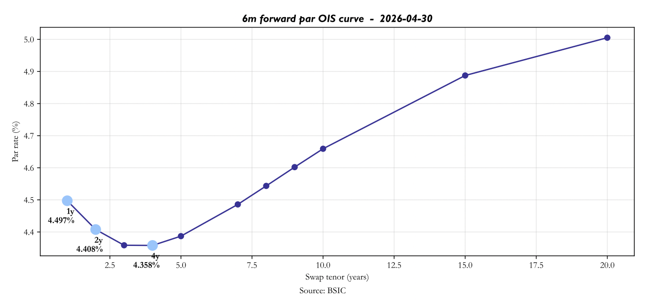
In our example with the best fly selected (6M 1Y/2Y/4Y) we have

$\boldsymbol{L} = \begin{pmatrix} 0.6960 & -0.5099 & -0.5055 \\ 0.6091 & 0.0464 & 0.7918 \\ 0.3802 & 0.8590 & -0.3429 \end{pmatrix}$ ,

where each row represents the tenor loadings on the 6m strip for each PCs (columns).

$\begin{bmatrix} 0.6960 & 0.3802 \\ -0.5099 & 0.8590 \end{bmatrix} \begin{pmatrix} w_{left} \\ w_{right} \end{pmatrix} = -100 \cdot \begin{pmatrix} 0.6091 \\ 0.0464 \end{pmatrix}$

Solving for the weights we have w_left (1Y)= -63.85, w_right (4Y)= -43.31 and belly (2Y)= 100.

Final Remarks

We note that the chosen candidate sits in a section of the GBP curve that is the most contested region of UK fixed income at the moment. On 28 February 2026 the United States and Iran moved into open hostilities affecting the Strait of Hormuz; Brent has rallied more than fifty percent since then and remains above $100 per barrel even after the most recent peace-deal headlines, with U.S. and Iranian forces exchanging fire as recently as 8 May. UK CPI, which had been expected to fall back toward the 2% target through the spring, instead jumped to 3.3% in March (from 3.0% in February), and the Bank of England’s own April Monetary Policy Report now projects CPI between 3.0 and 3.5 percent in Q2 and Q3 2026.

The MPC voted 8–1 on 29 April to hold Bank Rate at 3.75%, with the dissenter calling for an immediate hike to 4.00%; Governor Bailey described the policy environment as ‘the most difficult combination’ the Committee has had to face and explicitly declined to give forward guidance, saying the Bank ‘would not rush’ while the energy shock plays out. The cumulative repricing since hostilities began on 28 February has been pronounced: the SONIA-implied path that had priced roughly 50 basis points of cuts in 2026 before the war now prices roughly 60 basis points of cumulative hikes.

A Hormuz reopening coupled with a credible ceasefire, potentially dropping oil and LNG prices by 10-15%, could alleviate these tensions and allow the central bankers to see how these effects propagate through the supply chains and affect consumption transmitting in order through PPI, headline CPI and finally core CPI. On the other hand a sustained blockade with Brent at $130 or higher presents a different scenario with lower real rates which could significantly increase the pressure on the BOE to take actions. Both these scenarios are being averaged into a single forward curve that, in reality, is bimodal.

We believe that bimodality is precisely what stresses the curvature region of the 6m forward strip. The 6m1y forward (compounded SONIA between roughly six and eighteen months from today) sits in the segment where the bulk of any near-term hiking would appear, and so has repriced fastest and most cleanly. The 6m4y forward, extending into 2030–2031, instead anchors on the longer-run neutral rate plus a term-premium component that has been rebuilt by ongoing BoE quantitative tightening and by the broader gilt-market backdrop in which 30y yields have risen to 5.78%, the highest level since 1998. The 6m2y forward, by contrast, lives in the segment where the market would sit if the BoE hikes once or twice, then holds and is therefore the part of the curve most exposed to scenarios that depend on whether and when the energy shock is judged to be temporary. With Bailey explicitly refusing to anchor the medium-term path and the MPC visibly split (most split CB since the post-Covid); the result is a curvature pattern in which the wings have moved in lockstep with the broader policy-and-term-premium repricing, while the belly lags, leaving an isolated 2.4-σ residual on the trade-level basis that the PCA framework flags as cheap.

Therefore, the trade we recommend, is by construction neutral to a parallel shift in the curve and to a steepening or flattening, only profiting if the curvature of the 6m strip reverts toward the pattern implied by the last 261 days. Economically, this is a bet that the Iran-driven uncertainty resolves in either direction, with the market repricing the 6m2y point in line with the wings rather than continue to anchor it on a compromise level that reflects neither scenario. The model gives a signed rolldown of +3.54 bp per day on today’s curve against 0.79 bp of round-trip cost, but we do not treat this as the main reason to hold the trade. The rolldown is a rough approximation: it captures only the swap-tenor dimension, ignores the SONIA fixing leg, and is positive only because the 6m forward curve currently has a V-shape at the 2y point. The case for the trade rests on the residual dislocation and on the evidence of mean reversion in the recent regime.

We therefore treat the trade as regime-conditional and, given the geopolitical conditions, apply an eight-week review window of roughly four half-lives, by which time we would expect ~94% of the residual to have reverted under normal dynamics. The longer window is a deliberate choice in this regime: the dominant risk factor (the duration of the Iran-US conflict) operates on a multi-month rather than a multi-week timescale, and a tighter stop would force exits before either resolution path Hormuz: reopening or sustained blockade re-pricing has had time to play out.

References

[1] Cochrane, John H., Piazzesi, Monika, “Bond Risk Premia”, American Economic Review, 2005

[2] Kilian, Lutz, “Not All Oil Price Shocks Are Alike: Disentangling Demand and Supply Shocks in the Crude Oil Market”, American Economic Review, 2009

[3] Adrian, Tobias, Crump, Richard K., Moench, Emanuel, “Pricing the Term Structure with Linear Regressions”, Journal of Financial Economics, 2013

[4] Hanson, Samuel G., Stein, Jeremy C., “Monetary Policy and Long-Term Real Rates”, Journal of Financial Economics, 2015

Published by BSIC on 10 May 202610 May 2026

0 Comments

Leave a Reply Cancel reply

Market Recap 10/05/2026

A Physics – Based Model of Returns: Anomalous Scaling and Irreversibility

Relative Value in Rates: presenting and challenging the Gauss+ model