Introduction
The idea behind capital structure arbitrage is that the market pricing of equity and debt can diverge away from equilibrium, which might be because different types of investors are active in each market, and they possibly have different opinions about the prospects of a company. Therefore, capital structure arbitrage aims to generate profits by taking advantage of the misinformation between equity and debt markets, and the subsequent mispricing of a single issuer’s securities.
This form of arbitrage gained momentum at the start of the 21st century due to the expanding CDS market. The utilization of capital structure arbitrage by hedge funds surged significantly, rising by a factor of five from 2000 to 2005, with more than 300 active funds by the end of 2005.
A structural model, usually a variant of the Merton model (1974), uses equity prices to calculate the issuer’s credit default swap’s price. Based on the deviation of the model prices to the market prices, a convergence trading strategy is put to practice to take advantage of the theoretical price misalignment. If mispricing in the relative pricing between equity and CDS is detected, then depending on the direction of the mispricing an arbitrageur can either sell overvalued CDS protection and short equity as a hedge or buy undervalued CDS protection and buy equity. Of course, an arbitrageur will only make a profit if the prices of the instruments subsequently revert towards equilibrium, so a successful implementation of the strategy requires identifying mispricings that are on average corrected over some reasonably short time-horizon.
Capital structure arbitrage hinges on the issue of synchronization and the relative determination of prices in the equity, CDS, and bond markets. This is because sustainable gains from capital structure arbitrage can only materialize when there is an absence of full integration or variations in the speed at which these markets establish prices. Whenever disparities in pricing arise, they are typically rectified through adjustments in bond prices. Blanco et al. (2005) have observed that the CDS market is more responsive to alterations in firm-specific factors linked to credit risk, whereas the bond market reacts with a delay. That is likely due to greater liquidity of the CDS market and therefore using the CDS market in capital structure arbitrage is more cautious than using the bond market. Possible profits when using the bond market could be higher due to its arguably lower efficiency, but the traders’ ability to profit from bond mispricing would be limited by liquidity considerations.
Academic literature review
One of the first papers published on the topic was Fan Yu (2005), who examines the risks and returns of capital structure arbitrage using the CreditGrades model based on a sample of North American firms covering the period between 2001 and 2004. Yu (2005) analyzes strategies in several specifications with different holding periods (30 or 180 days) and different trading-triggers based on whether a deviation between the market and model CDS spreads exceeds 50%, 100% or 200%. He backtested the strategy using 4,044 daily CDS spreads on 33 obligors and found that individual capital structure arbitrage strategies are very risky and only 10% of the trades eventually converge. Yu (2005) also finds that while the mean holding period returns are negative or near-zero for the 30 day holding periods, they are positive for the 180 day strategy. The maximum mean holding period return of 2.78% is achieved for speculative grade obligors and the strategy using the 50% trading deviation trigger. However, after they conducted the statistical arbitrage test by Hogan et al. (2004), they found no evidence of significant arbitrage. A statistical arbitrage is defined by Hogan et al. (2004), as a zero initial cost self-financing trading strategy with positive expected discounted profits, a probability of loss converging to zero, and a time-average variance converging to zero.
The analysis of his trading returns (Yu, 2005) suggests that suggests that capital structure arbitrage works well when the market spread and theoretical spread follow each other closely. However, in his study Yu (2005) showed that across his data sample the correlation was -0.19, making it difficult to consistently profit overtime.
Duarte et al. (2007) find that capital structure arbitrage requires several times more capital to achieve a standard deviation of excess returns of 10%. They also find that these excess returns are positively skewed, meaning that investors may expect small frequent losses with few large wins.
Bajlum and Larsen (2008) reveal an intriguing finding: the profitability of capital structure arbitrage experiences a substantial boost when detecting relative mispricing between equity and debt using CreditGrades calibrated with option implied volatilities, as opposed to relying on historical volatilities. To illustrate this concept, they observe that the average returns over the holding period for speculative grade obligors rise from 2.64% to 4.61% when transitioning from historical to option-implied volatilities.
Wojtowicz (2017) obtained returns of 24.35% returns on an annual basis on a sample of American issuers, traded from 2010-12, however large standard deviations in the results continued being an issue, with results ranging from -109% to 336%, with a standard deviation of over 35%. The standard deviation is large compared to the mean holding period return implying that the mean return from the strategy can be substantially driven by outliers. In this study 65% of all trades were profitable, a large jump compared to previous studies conducted earlier in time. Wojtowicz (2017) found how returns in lower rated companies are higher when compared to higher rated companies. Furthermore, the standard deviations of the returns are higher the lower the rating category. It shows a clear trade-off between risks and returns of capital structure arbitrage with trades in the lower rated categories having higher returns, but also higher risks. It’s understandable that capital structure arbitrage yields relatively small profits for obligors with AA-AAA ratings because these companies typically have low CDS premiums. These premiums are primarily influenced by broader market dynamics rather than specific credit characteristics of individual firms.
Credit default swap
Credit default swaps (CDS), are over the counter financial contracts, which allow investors to manage their exposure to credit risk. In this swap contract, the seller compensates the buyer in the event of a credit event by the debtor. CDS can however also be used to express market views on the state of market entities’ credit story. In strategies like the one explored in this article, and other debt-equity strategies, the use of CDS is preferred to that of bonds, due to their higher liquidity. This is a possible alternative due to the mathematical relationship between CDS prices and their respective bond prices.
The Merton Model and CreditGrades model
As mentioned earlier, Merton (1974) was a revolutionary framework in the field of default probability research. Newer models have been developed but remain largely unchanged.
The CreditGrades model (1997) is a widely used structural model based on the Merton framework, which uses balance sheet data and market data in order to calculate CDS spreads. We will mention this model as we analyze a set of returns from Yu (2005), where the effectiveness of capital structure arbitrage is examined. In this section we will look at how the original model (Merton) predicts default probabilities, as it is the foundation for most models used industry wide nowadays.
The Merton model estimates default probability by comparing a company’s value to the face value of its debt. It utilizes option pricing theory in order to value corporate liabilities. Because the market value of the company which has debt, is not observable, the model infers it from the market value of the company’s equity. If the company’s debt is looked at as being a zero-coupon bond with maturity T, then the equity can be treated as a call option on the company’s value with the value of the company’s debt as a strike-price. In other words, at maturity, if the value of the company’s debt is superior to the company’s value, the investor would not exercise the call option, and hence the company would default, otherwise, the option would be exercised, allowing the investor to profit on the difference between the company’s value and that of its debt.
The value of the company’s equity can be expressed by the Black-Scholes option pricing equation. When the volatility of the company’s equity is fixed within a time period T, the value of the equity is:

Where E is the company’s equity value as a function of its value, V is company value, t is duration, r is the risk-free rate for the given duration t, D is the value of debt, and is the cumulative normal distribution and
are the option’s delta and probability of the option expiring in the money, respectively.
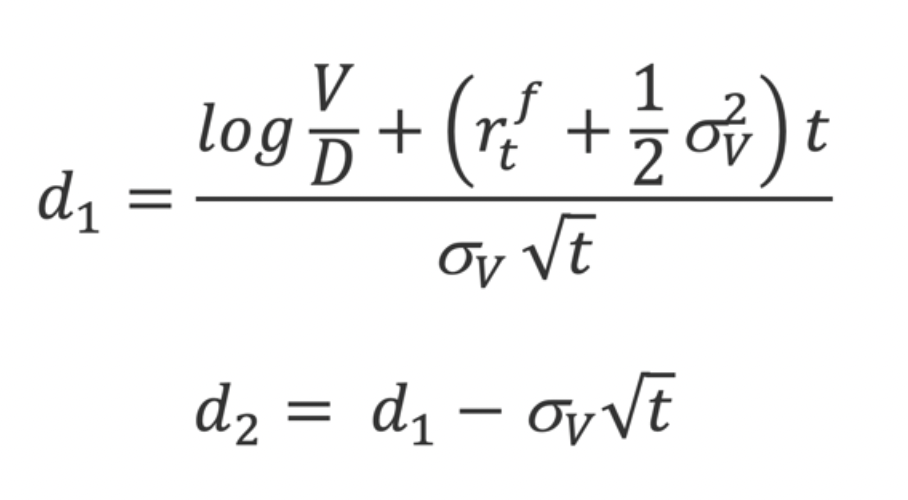
The equity’s volatility will then be:
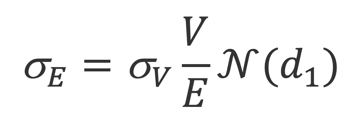
From here onwards, a solver determines the precise value of V and . Lastly, the distance to default and the probability of default of a given company with a typical t=1year horizon:
Probability of Default = N(-DD)
The main assumptions this model has, are that the company’s value V follows a Geometric Brownian motion, from time t to t+1, and that the probability of lying within the default area follows a Normal Distribution.
This Probability of Default allows us to derive the theoretical or model CDS prices, which are essential for the determination of the entry point of the trading strategy.
In all papers which will be mentioned in this article, the CreditGrades model (1997) will be used in order to detect the fair value of CDS spreads. The advantage of this model is that it provides closed-form formulas for the survival probabilities of obligors and also fair CDS premia levels that are functions of market observables. CreditGrades belongs to the class of structural models introduced by Black and Scholes (1973) and Merton (1974). According to these models both equity and debt can be viewed as options on the underlying firm value.
A problem with the application of the basic structure model is that it leads to a strong underestimation of short-term credit spreads. One commonly used strategy involves introducing jumps in the asset value progression, as demonstrated by Zhou in 2001, or integrating an internally determined default threshold, as exemplified by Leland and Toft in 1996. In contrast, CreditGrades opts for a more straightforward method by introducing an uncertain global recovery rate derived from a lognormal distribution.
CreditGrades posits a stochastic process that represents the asset value of the firm. is defined as a geometric Brownian motion with zero drift:
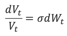
With being the Brownian motion and the asset volatility. The default threshold is assumed to be equal to the recovery given default, which in this case is (the product of the recovery on debt L and the amount of firm’s debt D).
The recovery rate is assumed to have a log normal distribution with mean and standard deviation such that . It is then assumed that where is the normal random variable independent of the asset value process. In this scenario, Z remains unknown until the moment of default, reflecting the uncertainty surrounding the firm’s debt level and the potential for an unexpected default event.
From this we can arrive to the survival probability of an obligor:
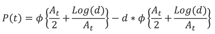
Where and are defined as follows:
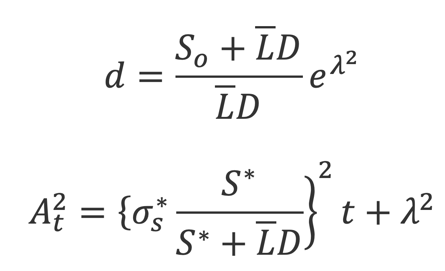
And all parameters are market observables, for example: is the initial stock price, is the reference stock price, is the reference stock volatility, is debt per share, is the mean of the global recovery rate and its standard deviation.
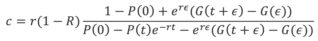
Given the probability of survival, the fair spread on a CDS can be obtained by equating the expected value of the default leg with the expected value of the premium leg. The fair CDS premia, denoted as “c” is the following:
CreditGrades (2002) furthermore specifies that you can obtain the asset volatility by rescaling the observable stock return volatility as follows:
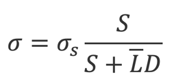
Where σs is the stock volatility, S is the stock price and LD is defined as previously. The equity volatility is typically computed as a long-term historical volatility based on past stock returns, while option-implied volatility can also be used and as shown higher returns are associated with using option-implied volatility.
Trading Strategy Mechanics
This section of the article focuses on the implementation of the trading strategy and possible outcome scenarios that can arise once the trade has been opened.
We assume that we have available a time-series of CDS market prices which we can denote as ct = c(t, t + ε)
We also assume that we have an analogous time series for equity prices which we can denote as St
If we denote the CDS price calculated with the structural model as c′t , we can denote the difference between these two time-series as et = ct − c′t
Studying the value we can derive the values and which are the mean and standard deviation respectively. These values are central to the trade’s entry and exit point. For example, the arbitrageur might find that the deviation has grown to an abnormally large value which could be > + 1.5 .
At this point the trader might consider the CDS to be overpriced, and decide to sell the credit protection instrument, with the supposition that convergence will occur, meaning market prices will adjust to the model prices. In this scenario, the trader should short the equity as a hedge due to the fact that there might be a case where despite the model’s predictions, CDSs are priced fairly, and that the equity market has been slow to react to new information. In this case the equity is overpriced, and one should short CDS as a hedge to shorting the equity. Clearly, both scenarios give rise to the same exact trade idea.
The size and nature of the equity hedge are factors which are at the discretion of the trader. However, there are some common practices and alternatives to approach this issue. The hedge is often static, meaning it remains unchanged throughout the duration of the trade. When it comes to the size of the hedge, a trader might increase or decrease the size from a predetermined model-based value depending on his conviction regarding convergence. On the other hand, some traders might elect to not use a model-based hedging ratio, and decide to quantify the size of their hedge, by calculating the maximum loss they can incur if the obligor defaults, and shorting an amount that would allow them to break-even.
What remains to be clarified, is the exit point of the trade, which occurs in two scenarios. Once the pricing difference has returned to near its mean value, or when a pre-determined holding period has elapsed. To limit losses, a trader might establish a ceiling for the value of
and close the trade once this value has been surpassed.
After the trade has been opened, there are four scenarios that can occur:
- and both decrease. In this case convergence occurs, hence the trader profits from both positions.
- decreases but increases. In this case the trader profits from his CDS position but yields a loss from his equity position. He will profit if the former falls more rapidly than the latter rises, giving place to partial convergence.
- increases but decreases. In this scenario, the trader profits from his equity position, but suffers a loss from selling the credit protection. He will profit if the former rises less rapidly than the latter decreases, giving place to another case of partial convergence.
- and both increase. In this case, divergence occurs, and the trader makes a loss on both positions regardless of the size of the equity hedge.
Risks of Trading Strategy
There are several possible reasons for ineffectiveness in this strategy, in this section we will aim to analyze the sources of this ineffectiveness, to better understand the poor returns that have been yielded historically.
Parameter misestimation can be an origin of losses in this trading strategy. Parameter misestimation can occur as a result of low frequency releases of data necessary for the model input. For example, the value of a company’s debt can vastly change since the last balance sheets were published, allowing for the model to predict CDS spreads which are not consistent with the current reality of the company at the time.
Large drawdowns are another point of concern when attempting to implement this trading strategy. The market does not absorb information at equal rates for all issuers. This can create an issue when establishing the predetermined maximum holding period for the trading strategy, as finding a value that fits most companies in a given sample is difficult. This results in the closing of positions at sub-optimal times, due to the fact that a position could have been closed, 15 days before convergence actually occurred, causing a loss that could have been avoided. This is one of the reasons that in Yu (2005) the strategy with a 180-day holding period yielded better results overall, but this comes with the inevitable price of possible large drawdowns, which might be a big issue, especially for institution investors.
A third source of negative or poor returns is model misspecification.
Conclusion
In conclusion, capital structure arbitrage is a model-based trading strategy which has risen to popularity in the past two decades, but has struggled to generate positive expected returns, according to Yu (2005). However, more recent research, particularly Wojtowicz (2017) shows that as the CDS markets continue to become more liquid, the trading strategy has become more profitable as a result of more attractive bid-ask spreads, with an annual return of 24.35%, on a sample of companies rated AAA-CC. The results also showcased that the strategy works best with poorer rated companies, with companies rated in the A’s category posting the poorest returns, and the companies in the C’s category responsible for the highest returns. However, even if some studies yield positive returns, one must not forget about the risks and drawdowns involved in this strategy. The most losses occurred when the arbitrageur shorts CDS and finds the market spread to be subsequently skyrocketing, at which point the hedging becomes ineffective and the CDS trading ceases forcing to liquidate the position.


0 Comments