Introduction
There is empirical evidence that index options, especially puts, are overpriced relative to individual stock options. Dispersion trading is a strategy aimed to capitalize from this mispricing. The aim of this article is to explore whether dispersion trading can still generate positive returns, but to generate a good trading strategy, we first need to understand the reasons for which the mispricing exists. We will thereby revisit what we published around 6 years ago in our 3-chapters trilogy Trading the Dispersion: chapter I.
Profitability of Dispersion Trading
There are two hypotheses on the source of the returns in dispersion trading; the first hypothesis argues that index options are more expensive compared to individual stock options because they bear the correlation premium (absent from individual stock options). The alternative hypothesis is that of market inefficiency, which argues that institutional options demand, as well as retail to some extent, and supply drive option premia to be higher.
Institutional changes in the options market in late 1999 and 2000 provide a natural experiment to distinguish between these hypotheses, since a fundamental market risk premium, such as the correlation premium, should not change as the market structure changes. The institutional changes that happened in the options market included cross-listing of options, the launch of the International Securities Exchange, a Justice Department investigation and settlement, and a marked reduction in bid-offer spreads. These changes reduced the costs for arbitraging potential pricing mismatches in index and single-stock options. Therefore, if the profitability of dispersion trading is due to mispricing of index options relative to equity options, one would expect the profitability of dispersion trading to decrease after the changes of the 2000s. In contrast, if the profitability of dispersion trading is due to compensation for a fundamental risk factor, the change in the option market structure should not affect the profitability of this strategy.
Deng (2008) found that dispersion trading was extremely profitable from 1996 to 2000, with average monthly returns of 24% with a Sharpe ratio of 1.2. However, the returns became negative after 2000, with the average monthly returns of -0.03% and a Sharpe ratio of -0.17. These findings provide evidence in support of the market inefficiency hypothesis and against the risk-based explanation.
One strand of literature argues that the differences in pricing of index and individual equity options is due to volatility risk and correlation risk, which are priced differently in index options and individual stock options. Bakshi, Kapadia, and Madan (2003) established a connection between the premiums of index options and individual options by highlighting the disparity in the risk-neutral skewness of the underlying distributions. Additionally, Bakshi and Kapadia (2003) provide evidence that the risk-neutral distributions for individual stocks differ from the market index. This distinction arises from the fact that the market volatility risk premium, although present in both individual and index options, is notably lower for individual options, and idiosyncratic volatility remains under-priced in single stock options. Recently, Driessen, Maenhout and Vilkov (2006), show that dispersion trading profits arise from a risk premium that index options have but is absent from individual options. This is the correlation risk premium, the difference between implied and realized correlation, which they claim is negatively priced, and since index options, especially index puts, hedge correlation risk, they are more expensive.
Another possible explanation for the overpricing in index options is the limitations or constraints of the market participants in selling options. According to Bollen and Whaley (2004), the net buying pressure present in the index options market drives the index options prices to be higher. Under ideal dynamic replication, an option’s price and implied volatility should not be affected no matter how large demand is. However, due to the limits of arbitrage, a market maker will never sell an unlimited amount of a certain option contracts at a given options premium. As he/she builds up the position in a certain option, his/her hedging costs and volatility-risk exposure also increase, and he/she is forced to charge a higher price. Bollen and Whaley also show that changes in the level of an option’s implied volatility are positively related to variations in demand for the option and argue that the demand for out-of-the-money puts (to hedge against stock market declines) pushes up implied volatilities on low strike options in the stock index options market. Furthermore, Garleanu, Pedersen and Poteshman (2006) complement Bollen and Whaley’s hypothesis by modelling options equilibrium prices as a function of the demand pressure. Their model shows how demand pressure in a particular option affects the implied volatility surface of the underlying. Empirical evidence shows how demand pattern for single-stock options is very different from that of index options, in fact it is proven that end users are net short single stock options but net long index options. Thus, single stock options appear cheaper, and their volatility smile is flatter compared to index options.
Correlation Risk Premium
As a market-wide increase in correlation has negative effects on institutional investors due to a lowered benefit of diversification, and that correlation between individual equities tends to dramatically increase in large market downturns, correlation risk would be most likely priced in index options especially in puts. Whilst individual options do not seem to possess negative variance risk premium, index options do. One way to explain the difference in pricing between individual as well as index options in terms of risk, would be a factor that affects a combination of individual assets whilst this risk factor would be missing from the individual ones. Ways to measure such a correlation risk would be either through measuring variance risk of an index vs. individual stock risks making up that index, through cross-sections of index and stock option returns, through comparing implied correlation from synthetic correlation swaps with realized correlation, and through dispersion trading itself.
Academic research has extensively shown that correlation risk is priced in. Possible explanations for it would be correlation levels having predictive power for market variance as in Merton’s ICAPM model, or a too high correlation risk premium caused by too much institutional and retail hedging demand and of a lack of arbitrage. One reason for it would be too large transaction costs of correlation strategies due to far higher bid-ask spreads experienced in individual options. One way to trade on implied correlation would also be correlation swaps, where realized correlation risks can be transferred to other investors, their pay-out is the difference between implied and realized correlation times a fixed amount.
Globally correlation risk premium has been shown to statistically significant at a 1% level in French, Swiss, German and US equity indices and at a 10% level for MSCI Pan-Euro Index, a global correlation risk premium has also been identified by using the weighted correlation risk premiums and has been shown to contribute more than 70% to cross-sectional equity index option returns for European and US indices. Average levels of correlation risk premiums have been shown to be higher in European equity indices compared to US indices, varying between
-1% and 19% for European markets vs 5% and 9% for the US for monthly maturities. This also means that the global correlation risk premium has a strong relationship with the returns of equity options. The economic uncertainty variable has been found to have significant effects on both broad indices as well as global correlation risk premium, while variance risk premium seems to be irrelevant.
Dispersion Trading Setup
Dispersion is a fundamental measure of risk in the stock market. It measures how differently stocks are performing relatively to the benchmark. In fact, the dispersion of an index is a measure of the collective behaviour of its components returns around their mean. We can say that the more each components returns deviates from the index returns, the more dispersed the index is. Correlation is extremely important to understand dispersion; for any given volatilities on the index components, the lower the overall correlation between them, the higher the dispersion of the index.
A long dispersion trade involves selling an ATM straddle on the index and buying ATM straddles on the components of the index. In addition, the whole option portfolio is hedged with a position in the underlying stocks, so that it is delta-neutral over the investment horizon. This strategy aims to profit from the fact that the implied volatility of index options tends to be relatively higher than the theoretical volatility calculated using components’ implied volatilities and betting on the convergence of the two as the options comes to expiry. Being long dispersion means that you want implied correlation to be lower than realized correlation, because you sell index options.
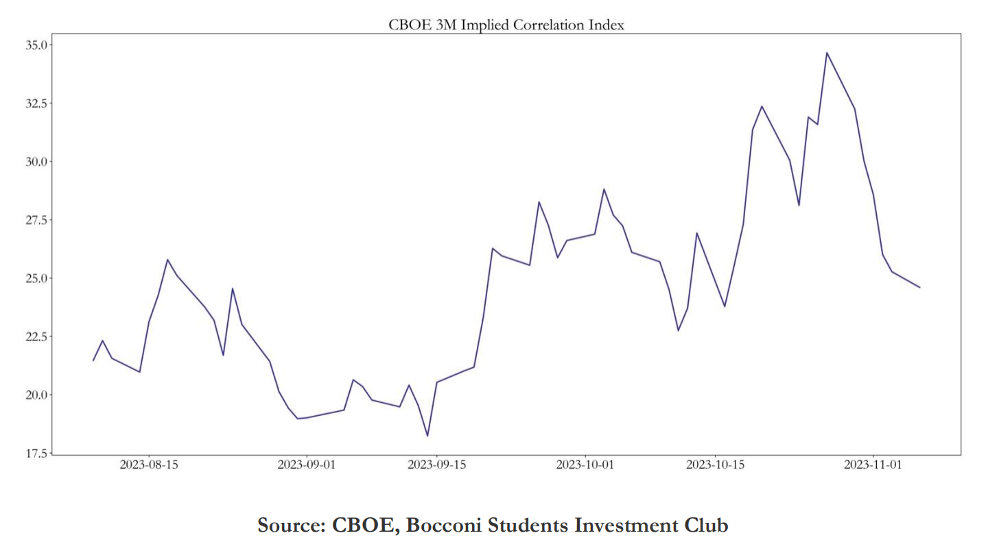
A tool that can help to time dispersion trades is the CBOE Implied Correlation Index. During the 2008-2009 Financial Crisis and the March 2020 COVID-19 crash, the dispersion resulted in a large increase in SPX implied volatility, without as a large increase in the component implied volatilities. This could have resulted in large profits if a trader was shorting dispersion, meaning that they want correlation to increase, profiting from a larger increase in the index implied volatility compared to the components implied volatilities.
Selecting a Subset of Index Components
To minimize trading costs for our strategy we seek to build a portfolio of stock options to trade that has less constituents than the index itself, as the main transaction costs arise from the single options legs of the trade. Especially when the positions are delta hedged, trading costs rise dramatically. The issue for trading less equity derivatives than equities included in the index itself is that it might cause issues as this basket of stock options might not be sufficiently representative of the index. When this is the case the exposure to the dispersion might not be as desired thus limiting potential profits as well as negating some of the reasons why would you enter the positions in the first place.
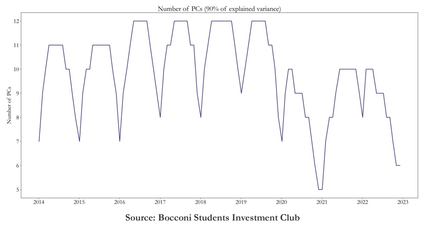
In order to create an optimal subset of index constituents, we used principal component analysis to determine the explanatory power of index variance for each constituent as in Schneider (2020). PCA is a method to reduce dimensionality in datasets through performing orthogonal linear transformation of data so that the first principal component inhibits the greatest variance with the following each with decreasing variance. This is done by first standardizing the initial variables as the PCA is sensitive with regards to the variances of the initial variables. A symmetric covariance matrix is then created to be able to determine the relationships between the variables as highly correlated variables have redundant information to some extent. By ranking the eigenvalues of this covariance matrix by descending order we are able to determine the eigenvector with highest amount of variance, and hence highest amount of. The percentage of variance accounted for by each eigenvector can then be computed by dividing their respective eigenvectors through the sum of eigenvalues. We start by computing the principal components that explain 90% of variance for all index members using the covariances of trailing one-year log returns, which gives us a certain number of principal components equal.
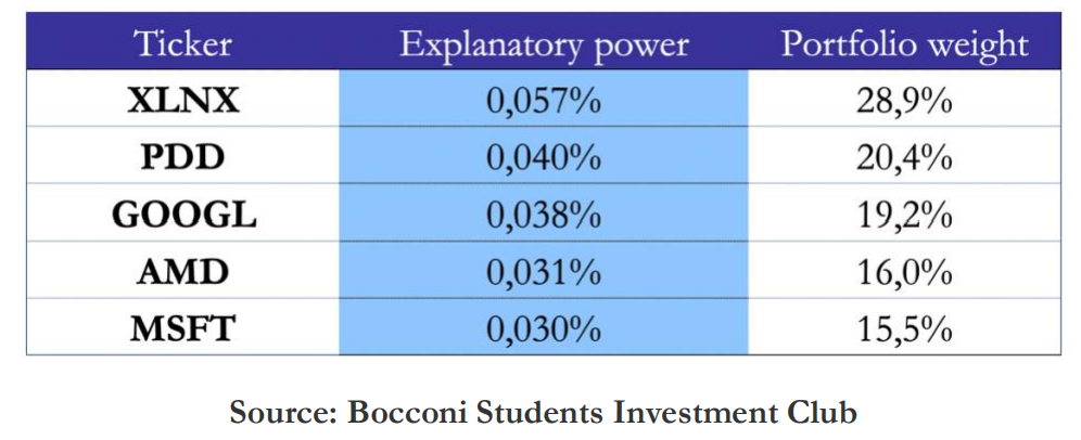
We then redo this step for every index member while omitting it to be able to compute the difference of the explained variance of the initial PCA with the reduced explained variance of the reduced PCA (omitting 1 index member). By performing this procedure for every stock, we can then select a number of stocks with the highest explanatory power. The weights of the stocks in the single-stocks options portfolio are then computed as ratio of the index member’s explained variation with the total explained variation of the selected stocks.
Set Up of the Trade
The ATM straddles of the single-stocks options are weighted according to the explanatory power of the PCA, and the whole single-stocks options portfolio is weighted against the index options to reach vega-neutrality. Vega-neutrality is important to hedge against the mis-pricing of correlation; when a dispersion trade is vega-weighted it can be thought as being the sum of the theta-weighted dispersion, which gives correlation exposure, combined with a long single-stock volatility position. In fact, this volatility exposure can be thought as being a hedge against a short correlation position (as volatility and correlation are correlated), thus giving greater exposure to the mis-pricing of correlation. Furthermore, it is empirically shown that the difference between single stock and index volatility (vega-weighted dispersion trade) is not correlated to volatility, which supports the view of vega-weighted dispersion being the best.

Conclusion
In this article we introduced dispersion trades, discusses the sources of their profitability, and explained a statistical method to select the single-stock options to trade against the index options. In the next article of this series we will show how to generate a signal to trade this strategy, together with its backtest.
References
- Bakshi, Kapadia, Madan, 2001. “Stock Return Characteristics, Skew Laws, and the Differential Pricing of Individual Equity Options”.
- Bollen, Whaley, 2004. “Does Net Buying Pressure Affect the Shape of Implied Volatility Functions?”.
- Garlenau, Pedersen, Poteshman, 2008. “Demand-Based Option Pricing”.
- Deng, 2008. “Volatility Dispersion Trading”.
- Driessen, Maenhout, Vilkov, 2009. “The Price of Correlation Risk: Evidence from Equity Options”.
- Schneider, Stübinger, 2020. “Dispersion Trading Based on the Explanatory Power of S&P 500 Stock Returns”.


0 Comments