Rough volatility: A Fractional Brownian Motion Approach.

Introduction

One of the biggest concerns regarding participants in the market is volatility. Through the years there have been different ways to model volatility in the market, starting with Black-Scholes that assumes constant volatility. Multiple major models have been developed at the scope of modelling volatility as a better reflection of reality. Examples are the Heston model, Jump-diffusion, local volatility. The aim of this article is to generalize even more the way volatility is modelled starting from a Volterra Process to obtain a Fractional Brownian motion (fBm), so that it better reflects what we observe in the markets. Additionally, we try to implement a trading strategy at the scope of testing the pricing power of the system. Through the rBergomi model which prices option through an fBm process we obtain the model’s volatility surface, which we use as a mean of finding mispricings along the market’s volatility surface. If triggered, we enter the trade through longing or shorting delta-hedged calls.

Volterra processes

A Volterra process is a specialized stochastic process defined as the integral of a time dependent Kernel with respect to a driving noise

$X_t = \int_{0}^{t} K(t,s) \, dW_s$

Where $K(t,s)$ is the Volterra Kernel and because it depends on the current evaluation at time t, it continuously re-weights as time moves forward, dictating the (auto)covariance structure of the process and allowing us to model the complex path-dependent autocorrelation structure

$\text{Cov}(X_s, X_t) = \gamma(s,t) = \mathbb{E}[(X_s - \mathbb{E}[X_s])(X_t - \mathbb{E}[X_t])]$

We know $\mathbb{E}[X_s] = \mathbb{E}[X_t] = 0$ as $W$ t is a standard Brownian motion

$\Rightarrow \gamma(s,t) = \mathbb{E}[X_s X_t] = \mathbb{E}\left[\int_{0}^{s} K(s,u) \, dW_u \int_{0}^{t} K(t,v) \, dW_v\right]$

Keeping in mind Ito Isometry

$\mathbb{E}\left[\int_{0}^{T} f(u) \, dW_u \int_{0}^{T} g(v) \, dW_v\right] = \mathbb{E}\left[\int_{0}^{T}\int_{0}^{T} f(u)g(v) \, dW_u \, dW_v\right]$

And considering that: $\mathbb{E}[dW_u \, dW_v] = \begin{cases} du, & u = v \\ 0, & u \neq v \end{cases}$

$\Rightarrow \int_{0}^{T}\int_{0}^{T} f(u)g(v) \, \mathbb{E}[dW_u \, dW_v] = \int_{0}^{T} f(u)g(u) \, du$

Applying it to our covariance function we have:

$\Rightarrow \gamma(s,t) = \mathbb{E}[X_s X_t] = \mathbb{E}\left[\int_{0}^{s} K(s,u) \, dW_u \int_{0}^{t} K(t,v) \, dW_v\right] = \int_{0}^{T} K(s,u) K(t,u) \, du$

Ultimately we have:

$\text{Cov}(X_t, X_u) = \mathbb{E}[X_t X_u] = \int_{0}^{\min(s,t)} K(s,u) K(t,u) \, du$

This formula shows that the kernel K fully determines the covariance structure of the process. Different choices of kernel produce processes with fundamentally different memory, regularity, and autocorrelation properties.

Standard and Fractional Brownian motion

Once we have defined the broad class of Volterra processes we can note that the case in which $K(t,s) = 1$ , the Volterra integral immediately simplifies to:

$X_t = \int_{0}^{t} 1 \, dW_s = W_t$

That is just a standard Brownian motion usually used to drive the noise in some notorious model like Heston, from empirical observations we can state that this structure is not sufficiently explanatory of some dynamics of the volatility observed in markets. Heston Model has the following dynamics:

$dS_t = \mu S_t \, dt + \sqrt{v_t} \, S_t \, dW_t^S$ (underlying)

$dv_t = \kappa(\theta - v_t) \, dt + \xi \sqrt{v_t} \, dW_t^v$ (volatility)

The volatility is driven by its own standard Brownian motion $dW_t^v$ which is correlated with the one of the underlying $dW_t^S$ . The parameters govern mean reversion speed ( $\kappa$ ), long-term variance ( $\theta$ ), and the volatility of volatility ( $\xi$ ). In this process, future evolutions depend only on the current state and do not incorporate information from the past. Comparing a visual representation of the volatility skew structure for ATM options given by the model and computed with a non-parametric estimate clearly shows why the model is not adequate to describe actual market dynamics.

The ATM skew (slope) at maturity $\tau$ is the derivative of the Black-Scholes implied volatility with respect to the log-moneyness evaluated at the money, practically measuring how fast implied volatility instantaneously varies as we move the strike away from the money.

$\psi(\tau) \coloneqq \left| \frac{\partial}{\partial k} \sigma_{BS}(k, \tau) \right|_{k=0}$

From the Heston model we can derive a closed form for the ATM skew, from which we can see that the Skew goes to zero linearly as $\tau \to 0$ and behaves as a sum of decaying exponentials for larger $\tau$

$\Psi_{\text{Heston}}(\tau) = \frac{\rho \xi}{2\sigma_0} \cdot \left(1 - \frac{1 - e^{-\kappa\tau}}{\kappa\tau}\right)$

Focusing on what happens at short maturities, we can expand the exponential for small $\kappa\tau$ and substituting we obtain:

$\Psi_{\text{Heston}}(\tau) \approx \frac{\rho \xi \kappa}{4\sigma_0} \tau \quad \text{as } \tau \to 0$

This behaviour is shown in the graph above. The other ATM skew along the term structure we can see in the graph, was computed on options data on the S&P500(SPX) from the same day 01/07/2020 but using instead a non-parametric estimate. Basically, we are not assuming any model we are just fitting the data locally. The procedure is as follows: for each expiry, we first estimate the forward price F using put-call parity across all strikes where both a call and a put are quoted. We then express each strike in terms of log-moneyness $k = \log(K/F)$ , which centers the smile around the forward. Keeping only options near the money (| $k$ | < 0.08), For each expiry, we fit a local quadratic $\sigma_{BS}(k) = a + bk + ck^2$ to the implied volatilities near the money. This is a second-order Taylor expansion of the implied volatility smile around the forward. The coefficient b represents the first derivative of implied volatility with respect to log-moneyness evaluated at $k$ = 0, which is precisely the ATM skew $\psi(\tau)$ . To assess the robustness of this approach and the structure it takes, we repeat the same procedures on different markets regimes.

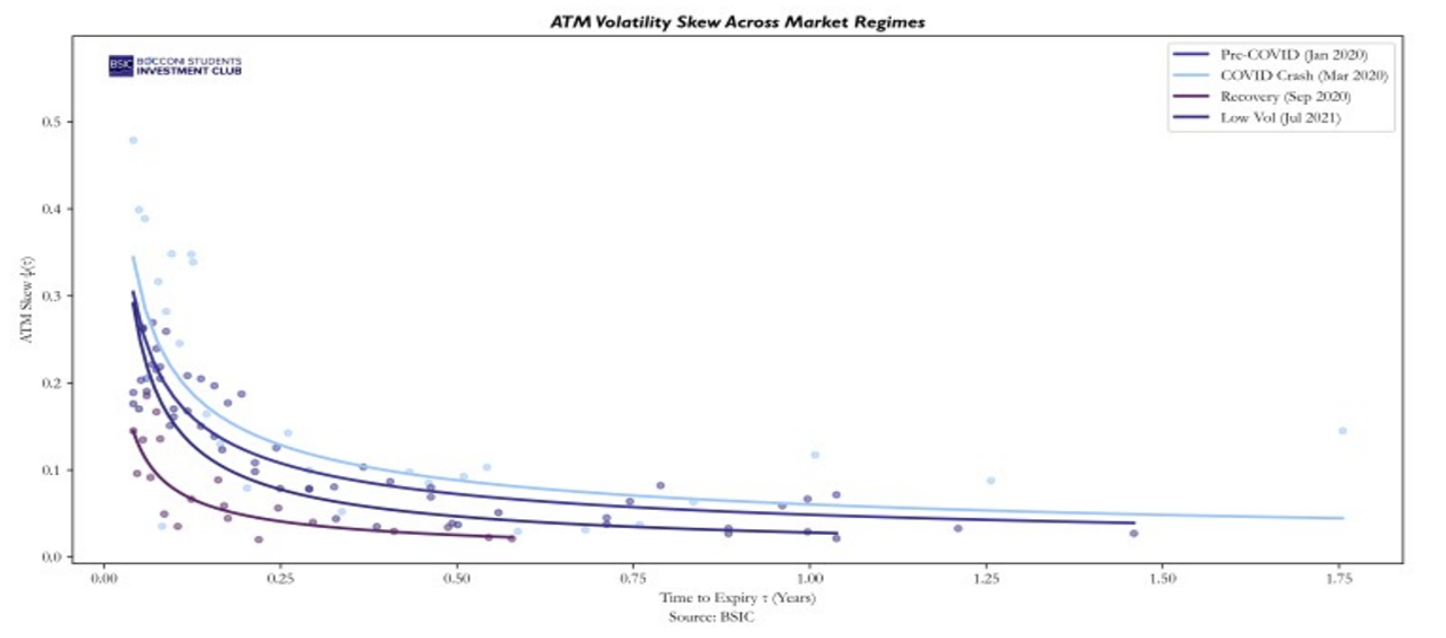We can confidently say that this is the shape that the ATM skew term structure takes, to try to fix the inconsistency of the Heston model with empirical observations we can’t consider $K(t,s) = 1$ , but instead a fractional Volterra kernel which generates a process called fractional Brownian motion (fBm). A fBm with $H \in (0,1)$ is a continuous centered Gaussian process that admits the Mandelbrot-Van Ness representation as a Volterra Integral, in fact choosing the Riemann-Liouville kernel:

$K(t,s) = \frac{(t-s)^{H-1/2}}{\Gamma\left(H + \frac{1}{2}\right)}$

We obtain

$W_t^H = \frac{1}{\Gamma\left(H + \frac{1}{2}\right)} \int_{0}^{t} (t-s)^{H-1/2} \, dW_s$

So the Covariance becomes:

$\text{Cov}(W_t^H, W_s^H) = \frac{1}{2}\left(t^{2H} + s^{2H} - |t-s|^{2H}\right)$

And we can observe that the covariance is fully determined by the parameter H.

Hurst parameter

We can clearly see that this process evaluated at time t , depends on H the Hurst parameter , when we have H =1/2 the exponent is 0 and we are back with the standard Brownian motion, in fact:

$\text{Cov}(W_t^{1/2}, W_s^{1/2}) = \frac{1}{2} \cdot 2s = s$

That is just $\min(s,t)$ , The most important feature of this formula is what happens to non-overlapping increments. Let us consider two consecutive, non-overlapping time steps of length $h$ : the past increment $W_h^H - W_0^H$ and the future increment $W_{2h}^H - W_h^H$ .By expanding the covariance of these two increments using our formula, it can be shown that the covariance between them is:

$\text{Cov}(W_{2h}^H - W_h^H, \; W_h^H - W_0^H) = \frac{1}{2} h^{2H} (2^{2H} - 2)$

This result clearly proves the existence of 3 different regimes:

When H = ½ then the term $2^{2H} - 2 = 0$ , proving that standard Bm has memoryless independently increments
When H> ½ then the term $2^{2H} - 2 > 0$ , proving the covariance is positive and the process trends
When H < ½ then the term $2^{2H} - 2 < 0$ , proving the process tends to mean-revert faster

is ju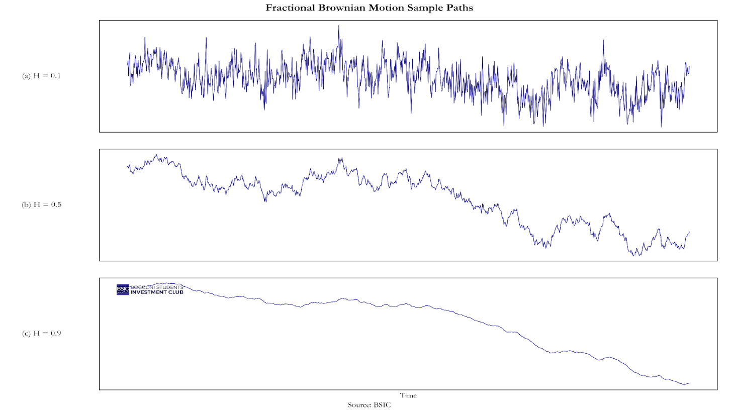Now we are interested in estimating what H is from empirical observation. To do that we start from log-volatility. If log-volatility behaves like fractional Brownian motion with Hurst parameter $H$ , then its increments satisfy a precise scaling law. For fBm:

$\mathbb{E}\left[|W_{t+\Delta}^H - W_t^H|^q\right] = K_q \cdot \Delta^{qH}$

Where $K_q$ is a constant that depends on $q$ but not on $\Delta$ so the $q$ -th moment of the increment scales as a power of the lag and the power is exactly $qH$ . Using data on SPY as a proxy of the S&P500, we compute realized volatility $\sigma_t$ from a 5-minute returns and then we take the log $x_t = \log(\sigma_t)$ . For each moment order $q \in \{0.5, \, 1, \, 1.5, \, 2, \, 3\}$ and each lag $\Delta = 1, 2, \ldots, \Delta_{\max}$ days, we compute the sample average:

$m(q, \Delta) = \frac{1}{N} \sum_{k=1}^{\lfloor N/\Delta \rfloor} |x_{k\Delta} - x_{(k-1)\Delta}|^q$

Then if the scaling law holds, we have:

$m(q, \Delta) \approx K_q \cdot \Delta^{\zeta_q}$

Taking logs:

$\log m(q, \Delta) = \log K_q + \zeta_q \cdot \log \Delta$

So for each $q$ , we regress $\log m(q, \Delta)$ on $\log \Delta$ . The slope of this regression gives us $\zeta_q$

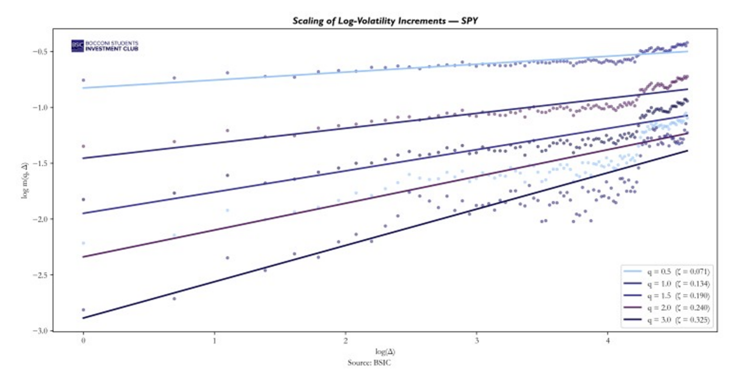
For each q, the data points lie along a straight line, confirming that the increments of log-volatility obey a power-law scaling. The slope of each line gives the scaling exponent $\zeta_q$ . Higher values of q produce steeper slopes, as expected since $\zeta_q = qH$ .

For fractional Brownian motion, the scaling exponents must satisfy $\zeta_q = qH$ .That is, they must be linear in q with slope equal to the Hurst parameter. To test this, we plot the estimated $\zeta_q$ against $q$ and fit a linear regression.

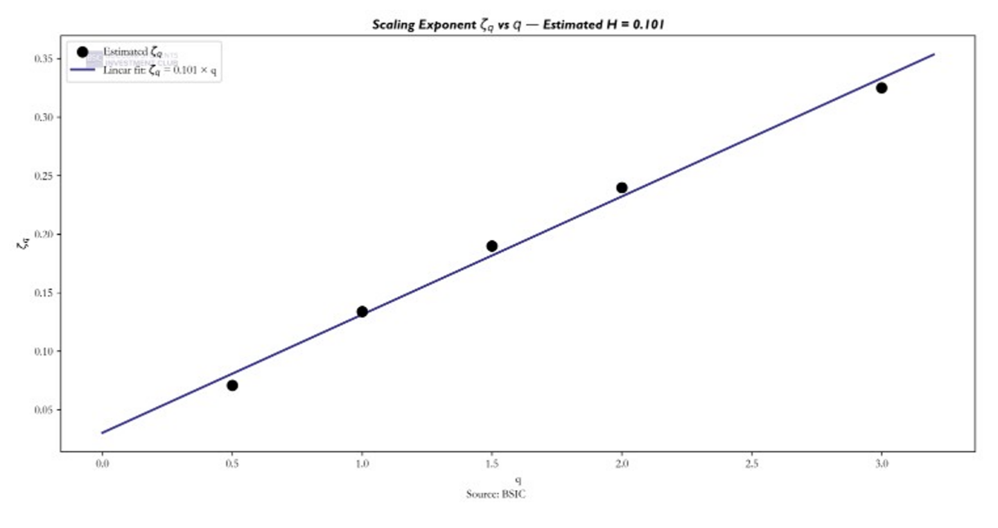The estimated exponents lie on a straight line with slope H = 0.101 and R² = 0.9924, confirming that log-volatility increments follow a monofractal scaling consistent with fBm, confirming that volatility is rough.

The estimated H ≈ 0.1 from the time series of realized volatility is independently confirmed by the options market. Fukasawa (2011) showed that under a stochastic volatility model driven by fractional Brownian motion, the ATM skew scales as $\psi(\tau) \propto \tau^{H-1/2}$ For H = 0.5, this gives $\psi(\tau) \propto \tau^{0}$ a constant, which is exactly the flat behavior we observed from the Heston model. For H = 0.1, it gives $\psi(\tau) \propto \tau^{-0.4}$ a power law that explodes at short maturities, matching the shape we observed in the non-parametric ATM skew plots on SPX data.

rBergomi pricing model

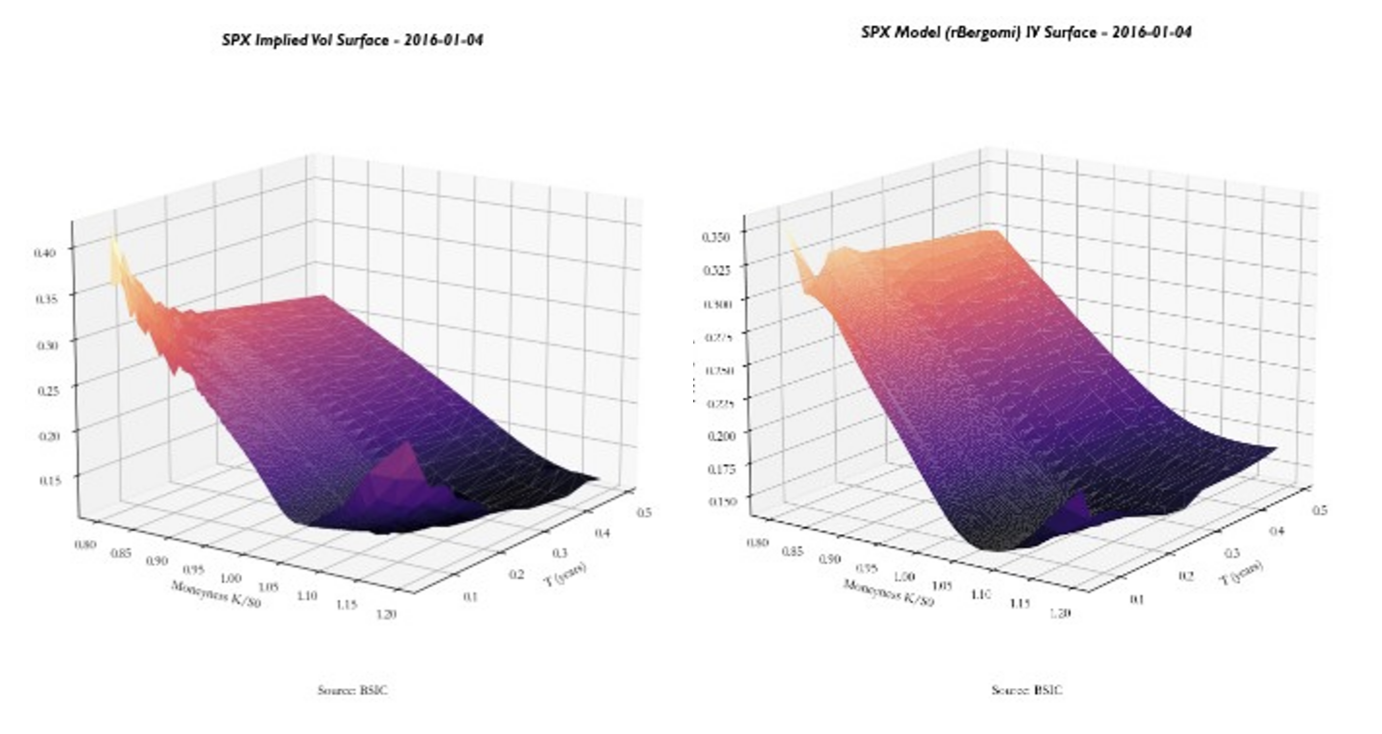
We now show how the fBm model can be used to price volatility across multiple strikes and maturities. We analyse in detail a simple case of this model, the rBergomi model, discussed in Pricing under rough volatility (2015). We expect that the rBergomi model fits the SPX volatility markedly better than conventional Markovian stochastic volatility models, and with fewer parameters.

Let’s now build the pricing model for SPX options through the rBergomi implementation. For this we will need to estimate four parameters: Forward Variance Curve ξ₀(t), Hurst parameter H, Correlation parameter ρ, Vol of vol η. These will be explained further in the article. Before detailing the calibration procedure, it is important to clarify the mechanism of the rBergomi model and how it generates option prices. The rBergomi model belongs to the class of rough fractional stochastic volatility (RFSV) models and is built upon three core components: A deterministic forward variance curve ξ₀(t), extracted from the market ATM term structure; A Volterra process driven by fractional Brownian motion, introducing roughness through the Hurst parameter H; A stochastic volatility structure controlled by the volatility-of-volatility parameter η and the spot–volatility correlation parameter ρ. In this way the model keeps the long memory characterizing the Volterra process and based on the degree of roughness (H), it gives more weight to the front-end part of the Term Structure.

In the rBergomi framework, the instantaneous variance process is defined as:

$v_t = \xi_0(t) \exp\left(\eta Y_t - \frac{1}{2} \eta^2 t^{2H}\right)$

where:

$Y_t = \int_{0}^{t} (t-s)^{H-\frac{1}{2}} \, dW_s$

is a Volterra Gaussian process.

The kernel (t-s)^H-1/2generates fractional behavior keeping a long memory through the Volterra process and introduces roughness in volatility paths through the Hurst parameter. Empirically, volatility exhibits short-term irregularity consistent with values H ~0.1, much lower than the classical Brownian case H=0.5, which gives a higher weight in the pricing process to recent maturities variance structures.

To simulate the model, a first Monte Carlo step generates the Brownian increments dW, The Volterra integral is computed numerically to obtain Y_t, the instantaneous variance paths v_t are constructed using the exponential representation above. This stage produces the full stochastic volatility dynamics.

Given the variance process, the underlying follows:

$\frac{dS_t}{S_t} = r(t) \, dt + \sqrt{v_t} \, dZ_t$

with:

$dZ_t = \rho \, dW_t + \sqrt{1 - \rho^2} \, dB_t$

where ρ controls the instantaneous correlation between spot and volatility shocks and is responsible for the implied volatility skew.

Once variance and spot paths are simulated, option prices are computed via a second Monte Carlo layer:

$C_{\text{model}}(K, T) = \mathbb{E}\left[(S_T - K)^+\right]$

The model-implied volatility surface is then obtained by inverting Black-Scholes prices.

Following, the parameters of the model are explained, and the estimation process is presented.

Forward Variance Curve – ξ₀(t)

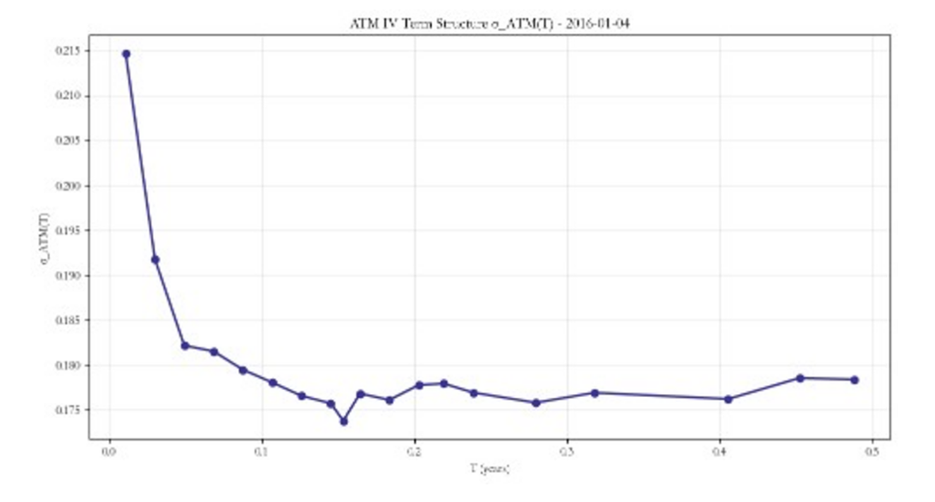
The forward variance curve ξ₀(t) is extracted directly from the market ATM term structure.

Starting from market ATM implied volatilities σ_ATM at different maturities we compute total variances:

$w(T) = \sigma_{\text{ATM}}^2(T) \cdot T$

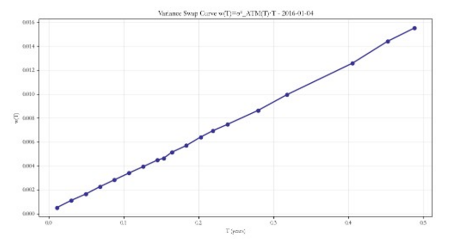
The instantaneous forward variance curve is then obtained via finite differences:

$\xi_0(t) \approx \frac{w(T_{i+1}) - w(T_i)}{T_{i+1} - T_i}$

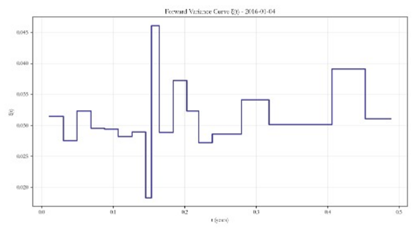
This is the base structure of our model which captures the implied volatility price by markets.

II: Hurst Parameter – H

The Hurst parameter, as explained in more detail previously, controls the roughness of volatility paths. Empirically, volatility exhibits rough behavior:

III. Correlation parameter (Volatility skew) – ρ

The parameter ρ represents the instantaneous correlation between spot and volatility shocks. It captures the leverage effect observed in equity markets: when ρ is negative, downward moves in the underlying tend to coincide with increases in volatility. This generates the characteristic downward sloping implied volatility skew across moneyness. A more negative ρ produces a steeper downside skew, therefore higher implied volatility for OTM puts and greater asymmetry in the return distribution.

Formally, ρ is the correlation between the Brownian motion driving the spot process and the Brownian motion driving the variance process:

$dZ_t = \rho \, dW_t + \sqrt{1 - \rho^2} \, dB_t$

where dWt drives volatility and dZt drives the spot dynamics.

Given ξ₀(t) and H, ρ is calibrated by minimizing the squared error between model implied option prices and market prices across selected strikes. The parameter assumes negative values and for the purpose of our article we will be fixing it at a value of -0.7.

Vol of vol (Volatility skew convexity) – η

The parameter η (eta) controls the amplitude of volatility fluctuations. It determines how strongly the variance process reacts to shocks and primarily affects the curvature (convexity) of the implied volatility smile. A higher η implies larger stochastic variance swings, fatter tails in the return distribution, stronger smile curvature. Importantly, η does not vary with maturity. However, the term structure effects arise from the interaction between η and the forward variance curve ξ₀(t)

Given ξ₀(t) and H, η is calibrated by minimizing:

$\eta^* = \arg\min_{\eta} \sum_{K} \left(C_{\text{model}}(K) - C_{\text{market}}(K)\right)^2$

In practice, η and ρ are jointly calibrated across the whole volatility surface through minimizing the squared error between the model σ_implied and market σ_implied, although due to heavy computational requirement for time constraints in our research we will be fixing ρ at -0.7 and calibrate η only. This is often preferred for numerical stability, and the rBergomi model is much more reliant on η accuracy than ρ.

Pricing reliability test through trading strategy implementation

The question at this point should be: does this pricing model give you an edge over the market? Well, it’s quite debatable. We present a backtest of our trading strategy that uses the rBergomi model to obtain the options pricing and then through reverse Black-Scholes obtains the model σ_implied along the volatility surface. By standardizing the difference between the model’s σ_implied and market’s σ_implied we identify mispricings and set our entry and exit thresholds. When triggered, each trade is opened through longing or shorting one delta-hedged call. We assume no transaction costs of any kind, and we use the mid-price to compute PnL between entry and exit, for simplicity reasons. It is very important to consider that our model is a very simplified version of the paper Pricing under rough volatility (2015) due to computational capacities. Therefore, we approximate ρ to -0.7 and we estimate η for each option through a grid search of η values ranging from 0.2 to 2.5 with 0.1 steps, through term-structures of three near-ATM strikes. The model is also exposed to many other variables other than volatility. Thus, the delta-hedging strategy doesn’t fully capture the essence of being only exposed to implied volatility, and the trading strategy test could fail to assess the reliability of the pricing.

Despite the previously stated condition, our backtest on options data ranging from 2015 to 2017 presents strong results.

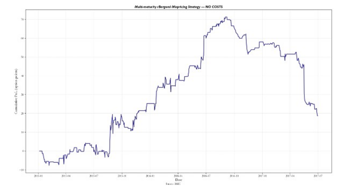
The model seems to work well until 2017 but as time progresses the pricing system loses its reliability and generates losses. For these reasons, we backtested it also from 2016 to 2025.

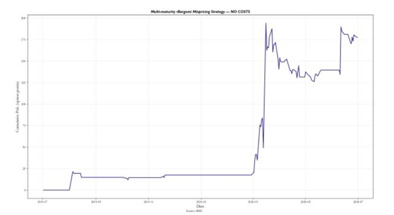
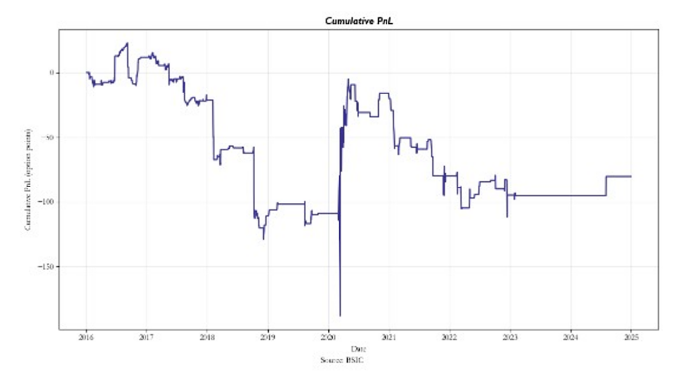The rBergomi fails thereafter. However, it is worth noting that in March 2020 the model delivered better options pricing than market ones, implying a stronger volatility modelling power during periods of crisis. Nonetheless, this could be mostly caused by statistical noise, and it could be an unreliable conclusion.

To this end we tested the model also in the 2008 financial crisis period resulting in:

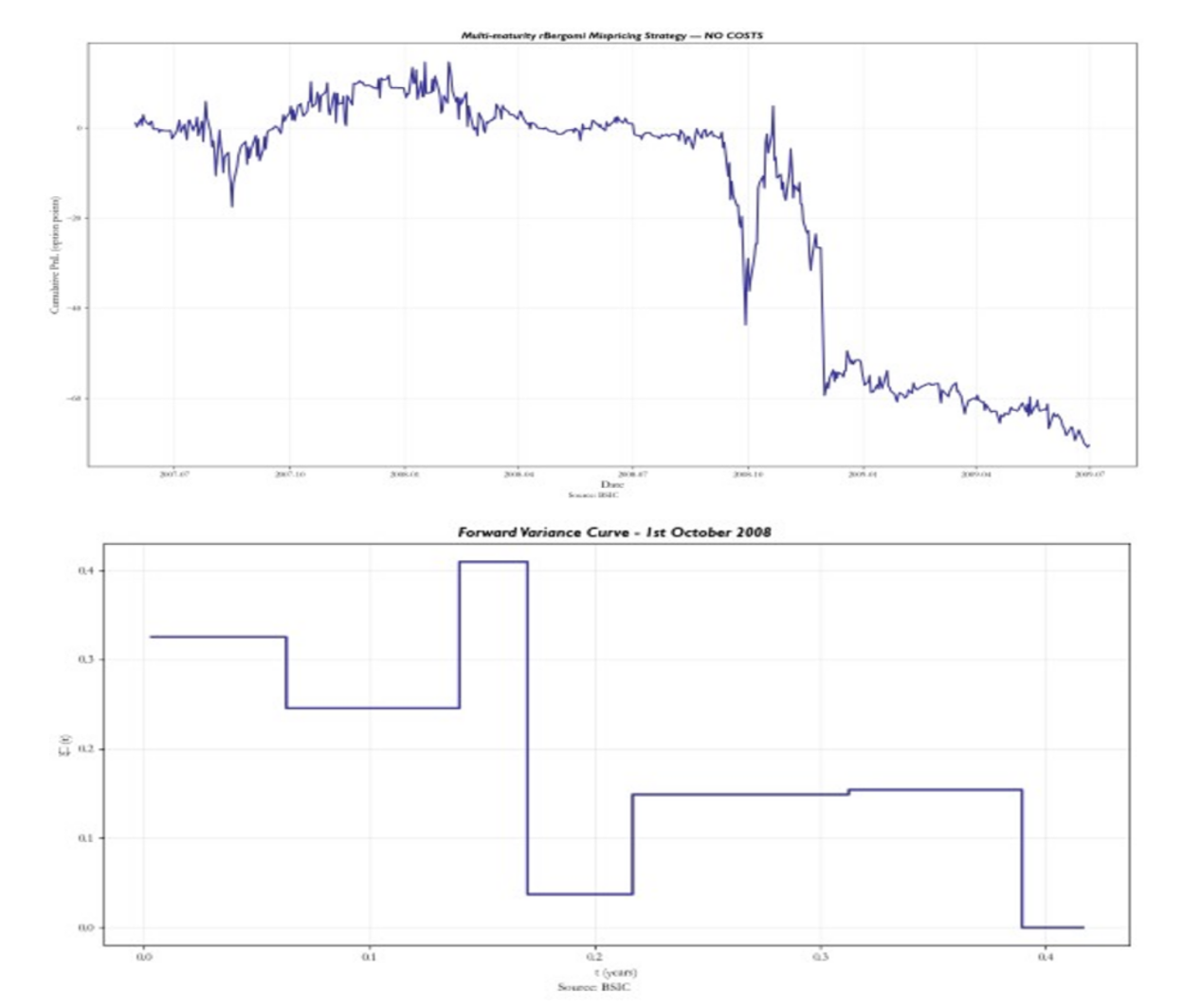
Notably, the model starts to produce PnL from the end of September 2008, right after the financial crisis beginning. The forward variance curve appears to be very irregular (rough) in the period. Thus, it further reinforces the idea that the model is very reliable in uncertainty periods. However, this statement is not sufficiently supported by our backtest, due to the lack of performance in other high stress periods and potential statistical noise which drove the returns.

The reliability of the model cannot be discarded though, and the reason behind the performance breakdown, outside of the period associated with the Pricing under rough volatility (2015) publication, could be caused by the assumptions we made on the fixing of parameters we extrapolated from the paper results, calibrated in line with the period 2015-2017. Finally, given our parameters estimation, the strategy seems to be having an edge in high financial stress periods right after the crashes, like October 2008 and March 2020, while it loses its pricing power outside of these events.

Conclusion

The empirical evidence presented throughout this article strongly supports the rough volatility paradigm. By estimating the scaling behaviour of log-volatility increments, we find that the Hurst parameter is significantly below the Brownian benchmark of H = 1/2, confirming that volatility exhibits persistent roughness and short-term irregularity. This stylized fact is consistent across datasets and aligns with literature on fractional volatility dynamics. Building on this empirical foundation, we implemented the rBergomi model as a tractable rough stochastic volatility framework. The model combines three structural components: a deterministic forward variance curve extracted from the market, a Volterra process driven by fractional Brownian motion, and a stochastic volatility structure governed by the volatility-of-volatility parameter η and the correlation parameter ρ. Together, these ingredients allow the model to capture the steep short-maturity skew and convexity patterns that standard Markovian models such as Heston fail to reproduce. The comparison between market-implied and model-implied volatility surfaces highlights the structural advantage of rBergomi in reproducing front-end skew behaviour. The model is particularly effective in stress regimes, where volatility dynamics become more irregular and the forward variance curve displays strong non-linearities. This suggests that roughness is not merely a theoretical refinement but a relevant feature of financial markets, especially during periods of heightened uncertainty. However, the trading implementation reveals important limitations. While the strategy based on model-implied mispricings performs well in certain periods notably around crisis episodes its performance deteriorates in calmer regimes. This instability likely reflects both model misspecification outside stress environments and the simplifying assumptions adopted in calibration. Moreover, the delta-hedged structure does not isolate pure volatility exposure and may introduce residual risk components. Rough volatility captures essential short-term market features, but translating structural accuracy into stable trading performance remains challenging. In conclusion, rough volatility offers a compelling lens through which to reinterpret implied volatility dynamics. The rBergomi model demonstrates that incorporating fractional behaviour materially improves structural fit, yet practical implementation requires careful calibration, risk control, and regime awareness.

References

[1] Gatheral, J., Jaisson, T. and Rosenbaum, M. (2018). ‘Volatility is rough.’ Quantitative Finance, 18(6),

[2] Fukasawa, M. (2011). ‘Asymptotic analysis for stochastic volatility: martingale expansion.’ Finance and Stochastics, 15(4)

[3] Bayer, C., Friz, P. and Gatheral, J. (2016). ‘Pricing under rough volatility.’ Quantitative Finance, 16(6)

Published by BSIC on 1 March 20261 March 2026

0 Comments

Leave a Reply Cancel reply

Technical Analysis on Steroids

Market Recap 01/03/2026

Market Recap 22/02/2026