A Practical Guide to Pricing Weather Derivatives

Introduction

Weather conditions play a fundamental role in the dynamics of the world economy, with estimates revealing that nearly 30% of economic activities and an overwhelming 70% of businesses encounter susceptibility to weather-related fluctuations. This substantial impact underlines the critical necessity to hedge the risk associated with weather. Among these strategies, weather derivatives emerge as a powerful tool, enabling market participants to effectively mitigate the adverse effects of weather variability on their operational efficiencies and financial performance.

Market Participants and Purposes

The history behind the development of weather derivatives relates to the deregulation of energy markets in the late 1990s. Previously, energy companies operated under monopolistic conditions, playing multiple roles such as production and distribution, and could easily shift the burden of unexpected weather-related costs to consumers. However, deregulation led these companies into a competitive landscape, which significantly increased the demand for ways to hedge against weather-related risks. In seeking solutions, energy companies turned to the capital markets. This search culminated in the creation of weather derivatives in 1997, an innovative financial tool designed to mitigate the financial uncertainties caused by unpredictable weather patterns.

It is relevant to mention that weather derivatives have not emerged to replace traditional ways of insurance. Weather derivatives are designed to manage the financial impact of predictable, moderate weather events, such as mild winters or cool summers, as opposed to insurance, which typically covers less frequent, high-impact events like hurricanes or blizzards. The payout mechanism of weather derivatives is directly linked to the magnitude of the weather event, allowing for proportional compensation, whereas insurance payouts are generally fixed amounts contingent upon proving a financial loss. This fundamental difference streamlines the claims process for weather derivatives, reducing the need for extensive documentation and legal proceedings. Additionally, weather derivatives are tradeable securities, offering companies the flexibility to buy or sell coverage based on changing risk assessments or weather forecasts. This contrasts with traditional insurance policies, which are usually non-transferable contracts between the insurer and the insured.

In general, there exist two standard ways to trade weather derivatives. The first one takes into consideration the primary market where weather hedges are provided for end-users that face weather risk in their business. In the US, most derivatives are traded at CME where both options and futures are provided for a wide range of the US and European cities. Besides the primary markets, there exists the opportunity to trade weather derivatives on secondary markets. Several counterparties, among which insurance companies, commercial banks or energy merchants belong, may be willing to assume the weather risk exposure of an energy company.

Categories of Weather Derivatives

Much of the weather market is dominated by temperature derivatives, aimed to protect the holder from unexpected temperature prints. The underlying used to trade these contracts is either Heating Degree Days (HDD) or Cooling Degree Days (CDD). For a specific day n, these can be defined as:

$\begin{aligned} & H D D_n=\max \left(T_{\text {ref }}-T_n, 0\right) \\ & C D D_n=\max \left(T_n-T_{r e f}, 0\right)\end{aligned}$

where $T_ref$ is a reference temperature and $T_n$ is the temperature of day n, conventionally computed as the mean between the minimum and maximum temperature recorded in the day. The most popular temperature instruments traded are options, whose payoff function depends on a cumulative sum over a longer period, usually an entire season:

Heating Degree seasons: $D D=H_P=\sum H D D_n$

Cooling Degree seasons: $D D=C_P=\sum C D D_n$

The payoff of a call option is therefore equal to $\propto * \max (D D-K, 0)$ and the payoff of a put option is equal to $\propto * \max (K-D D, 0)$ where K is the strike price and is the payment per degree day, commonly equal to $2500 or $5000.

Figure 1: Different option types, MPRA Paper 35037, BSIC

Other types of weather derivatives include rainfall contracts, measured in inches, and offered for trading by CME on a monthly or seasonal basis from March to October; snowfall contracts, also measured in inches and offered for trading by CME on a monthly or seasonal basis from November through April; and wind derivatives, which depend on the daily average wind speed measured by a predefined meteorological station over a specified period. However, interest for these products is purely demand driven and is generally initiated by a client wishing to protect against unfavourable weather conditions. The main reason is that precipitations and wind speed are harder to model than temperature, adding to the fact that the former is supplied only during specific seasons. Two other issues that represent a drawback for demand are geographical and basis risk: the first one results from the distance between the company that wishes to hedge and the station at which the weather measurement takes place, while the latter arises from the relationship between the hedged volume and the underlying weather index – the payoff of the contract is based on the weather index and it is unlikely to compensate for all the financial losses.

A Practical Pricing Process: Temperature Options – Sidney

In this section, we aim to provide a practical guide to pricing temperature options using Sidney weather data, consisting of the highest and lowest temperatures recorded each day for the past 165 years.

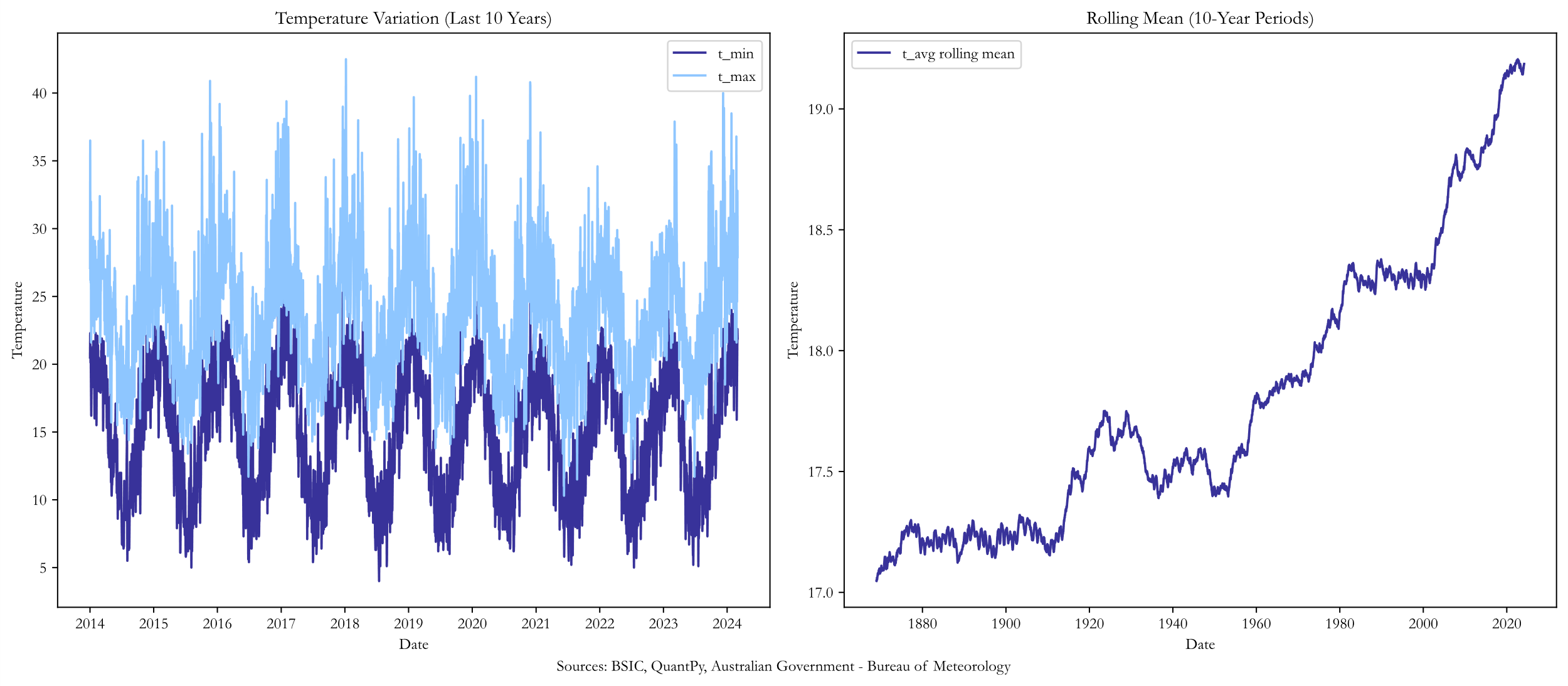
As can be observed from the graphs, there are trend and seasonality components in the data that must be filtered out before we start pricing the options. We must undertake a few steps in modelling Daily Average Temperature (DAT): de-trending and removing the seasonality from the raw data, using the filtered time series to model temperature, selecting the method with which we will model the temperature volatility, and finally using these models to price an option. We dive into each of these steps by providing the mathematical intuition behind it and going over our results.

1. Modelling Seasonality

The first step in pricing temperature options is to decompose the time series into several components, each representing an underlying pattern category. This can be represented as:

$y_t=T_t+S_t+e_t$

where $T_t$ represents the trend, $S_t$ represents the seasonality and $e_t$ represent the variability or noise, at time step t.

One of the most widely used methods is classical decomposition – calculating the trend-cycle component $\widehat{T}_t$ using a MA model, then estimating the seasonal component by averaging the detrended values for each season and finally computing the remainder by subtracting the first two components – however, this approach presents a few drawbacks, especially when analysing longer series, such as over-smoothing rapid rises and falls in the data, the wrong assumption that the seasonal component repeats from year to year, not accounting for the first few and last few observations when estimating the trend cycle and presenting significant autocorrelation within the error terms.

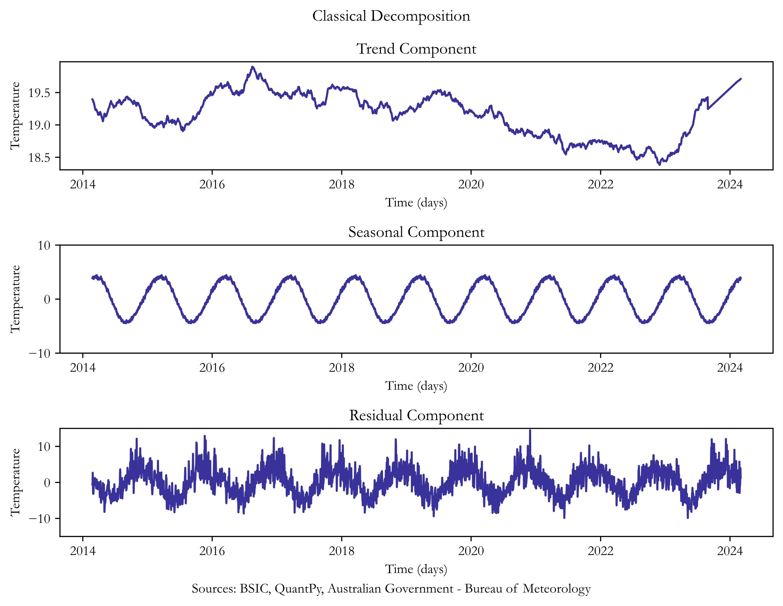
It is clear that the residual component exhibits substantial autocorrelation, thus we would use a more suitable approach, involving the use of Fourier series. The model for deterministic seasonal mean temperature is:

$\overline{T_t}=T_{\text {trend }}+T_{\text {seasonal }}$

where $\overline{T_t}$ represents the average temperature.

To observe trend and overall peaks, the DAT series must be firstly denoised, as the data presents a lot of variation in noise. Afterwards, by plotting a rolling mean over annual periods, a linear long-term trend is observed, thus $T_{\text {trend }}$ could be approximated by $T_{\text {trend }}=a+b t$ . As for the seasonal component, a simplified version of first order Fourier series, using a single sine function, is able to capture all the information and avoids overfitting:

$T_{\text {seasonal }}=\alpha * \sin (\omega t+\theta)$

The speed of the seasonal process should be assumed to be $\omega=\frac{2 \pi}{365.25}$ to account for the fact that an additional value is counted once every 4 years, especially when using longer time series. To fit the model, we use a non-linear least square that minimizes the sum of the squared deviations:

$\hat{\beta} \in \operatorname{argmin}_\beta S(\beta) \equiv \operatorname{argmin}_\beta \sum_{i=1}^N\left[y_i-f\left(x_i, \beta\right)\right]^2$

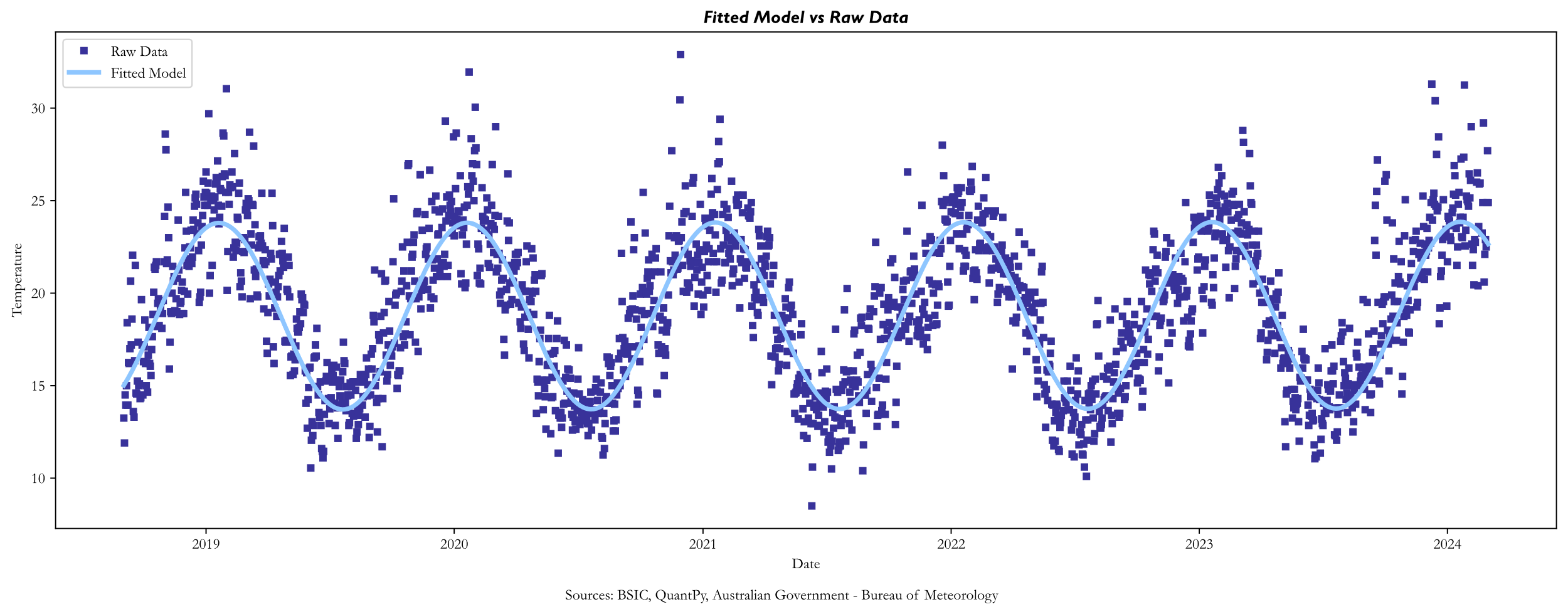
The model obtained for the deterministic seasonal mean temperature is:

$\overline{T_t}=16.8+(3.34 e-05) t+5.04 * \sin \left(\frac{2 \pi}{365.25} t+1.27\right)$

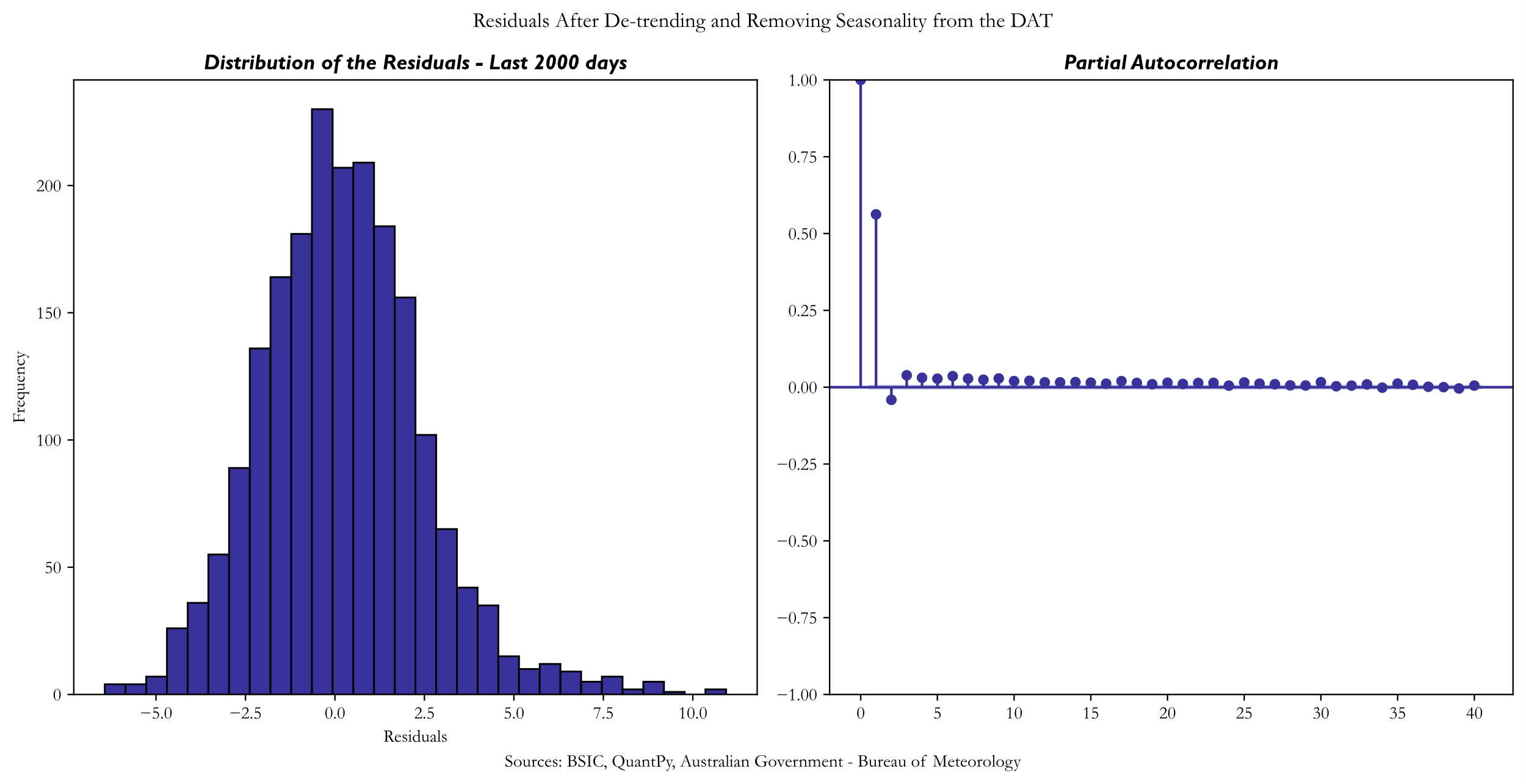
The first issue that appears when fitting the model to our data is a strong partial autocorrelation identified at the first-time lag, when analysing the residuals. Moreover, by plotting the residuals distribution against the quantiles of a normal distribution, we notice an upside deviation from the normal on the right tail of the distribution. However, it indicates that we should fit an Autoregressive model with 1 time lag for the error term, that will help us in the next step.

2. Modelling Temperature

To model the variation of the estimated temperature model, we need to fit a mean-reverting stochastic process, with the most widely used by literature being an Ornstein-Uhlenbeck (OU) continuous process. The use of a mean-reverting one is justified by the cyclical nature of temperature. An essential condition that must hold in order to capture the mean-reverting dynamics of temperature is $E\left[T_t\right] \approx \bar{T}_t$ . In our case, however, this condition is violated for a general OU process, that can be described as:

$d T_t=\kappa *\left(\bar{T}_t-T_t\right) d t+\sigma_t d W_t$

where is the mean-reversion parameter. To solve this stochastic differential equation (SDE), Ito-Doeblin formula is required, that is, for an Ito process x:

$d f(t, x)=f_t(t, x) d t+f_x(t, x) d x+\frac{1}{2} f_{x x}(t, x) d x d x$

The best function to use is an exponential one with the mean-reverting parameter with respect to time, multiplied by the Ito process: $f(t, x)=e^{\kappa t} * x$ , where $f_t(t, x)=\kappa * e^{\kappa t} * x, f_x(t, x)=e^{\kappa t}$ and $f_{x x}(t, x)=0$ . An exponential function is best suited to solve a normal (non-stochastic) integral by the integrating factor method. Applying the Ito-Doeblin formula for our Ito process, with dynamics d described by the general OU process, we obtain:

$\left d(e^{\kappa t} T_t\right)=\kappa * e^{\kappa t} \bar{T}_t d t+e^{\kappa t} \sigma_t d W_t$

Taking the integral over a given unit of time $u \in[s, t]$ , where $t>s$ , and changing the base on the Riemann integral to $d \overline{T_t}$ , will give us a final solution for temperature of:

$T_t=\bar{T}_t+\left(T_s-\overline{T_s}\right) * e^{-\kappa(t-s)}+\int_s^t e^{-\kappa(t-s)} \sigma_t d W_u$

whose expectation is not equal to the long-run average. This happens because the mean process that the equation is reverting to, $\bar{T}_t$ , is not constant over time and changes from one time step to another. A solution to this issue is incorporating the AR(1) term from the previous point, where we noticed partial autocorrelation of error terms for one time lag. Specifically, we will add the change in the seasonally adjusted mean, $\frac{d \overline{T_t}}{d t}$ , to our drift rate so that the long run mean of the SDE is $\bar{T}_t$ .

$d T_t=\left[\frac{d \overline{T_t}}{d t}+\kappa *\left(\overline{T_t}-T_t\right)\right]+\sigma_t d W_t$

3. Estimating the Speed of the Mean-Reversion Process and Volatility

To estimate the mean-reversion parameter, we use an Euler discretization of the SDE over a time interval $t \in[i-1, i]$ , that can be represented as follows:

$T_i-T_{i-1}=\bar{T}_i-\bar{T}_{i-1}+\kappa *\left(\bar{T}_{i-1}-T_i\right)+\sigma_i * z_i$

where $z_i \sim N(0,1)$ . Denoting $\widehat{T}_t=T_t-\bar{T}_t$ , we obtain $\widehat{T}_i=\widehat{T}_{i-1}-\kappa * \widehat{T}_{i-1}+\sigma_i * z_i$ , which can be modelled as an $\mathrm{AR}(1)$ process:

$\widehat{T}_i=\gamma * \widehat{T}_{i-1}+e_i$

where we denoted $\gamma=1-\kappa$ and $e_i=\sigma_i * z_i$ . After fitting our $\mathrm{AR}(1)$ model, we obtain an estimate of $\gamma=0.5625$ , so $\kappa=0.4375$ .

Since the standard deviation of temperature is non-constant over time, we would also need to find an equation that would best approximate the volatility component in the Ornstein-Uhlenbeck (OU) continuous process.

The method that we found most suitable for this job is B-spline (because of its smoothing properties), a curve approximation, which estimates unknown data points in each range. This approach requires the following parameters: knots (joints of polynomial segments), spline coefficients and the degree of a spline. We now plot B-spline curve approximations against the standard deviation of the temperature, for different numbers of knots, measuring the residual sum of squares (RSS), for every single one of them. This would help us with the choice of knots for our final model.

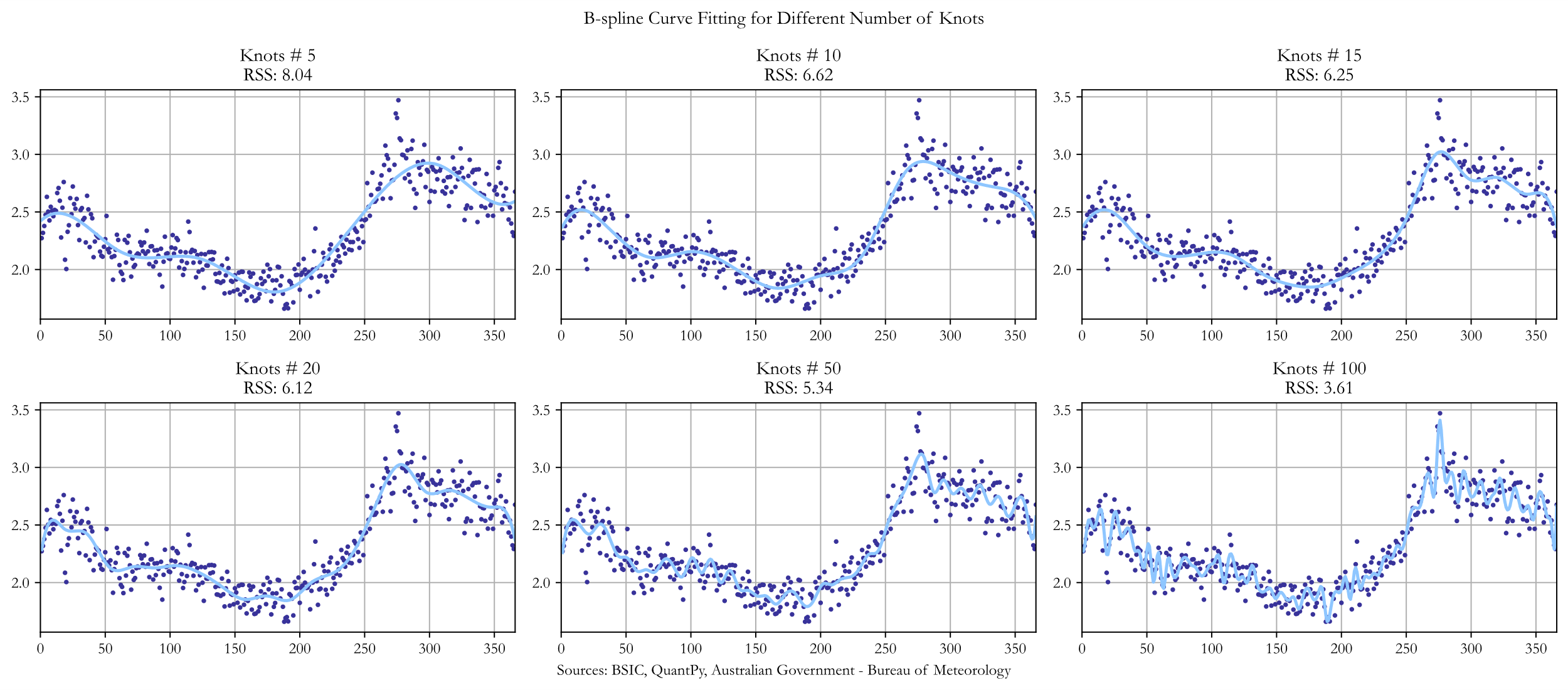
We observe that the RSS does not change substantially when including more than 10 knots, while the model seems to exhibit substantial overfitting. Since we want to present a robust pricing model, we chose to use 10 knots for our final approximation.

A more systematic, and reliable way to choose the number of knots could involve an optimization of the relationship between RSS and some overfitting measure, which is not within the scope of this article.

4. Monte Carlo simulations of temperature data

To simulate temperature data, we firstly define our approximation using a Euler scheme:

$T_{i+1}=T_i+\bar{T}_i^{\prime}+\kappa *\left(\bar{T}_i-T_i\right)+\sigma_i z_i$

We then define a Monte Carlo function that takes as inputs the trading dates in which temperature is to be forecasted, the number of simulations, the parameters of the OU process obtained above, the fitted volatility model, the first ordinal of the $\bar{T}_t$ model and the mean-reverting parameter obtained above. The function returns as output two dataframes, one that contains all the individual components resulted and the other one including all the simulated temperature paths for each specific trading day.

5. Risk Neutral Pricing of Temperature Options

For our risk neutral pricing, we are going to use the already mentioned Ornstein-Uhlenbeck (OU) model for the variation of the estimated temperature, and we will use the B-spline interpolation to describe the non-constant volatility term of the OU model. In this section, we will compare two pricing methods, a Black-Scholes approximation and a Monte Carlo approximation when pricing a winter Sidney call option. It is important to clarify that Australia’s winter period is from June to August. We use the 10Y Australian bond yield as a proxy for the risk-free rate, approximately equal to $r=0.041$ , a strike price of cumulative degree days equal to $K=300$ and a tick per degree day of $\propto\ = \$2500$ .

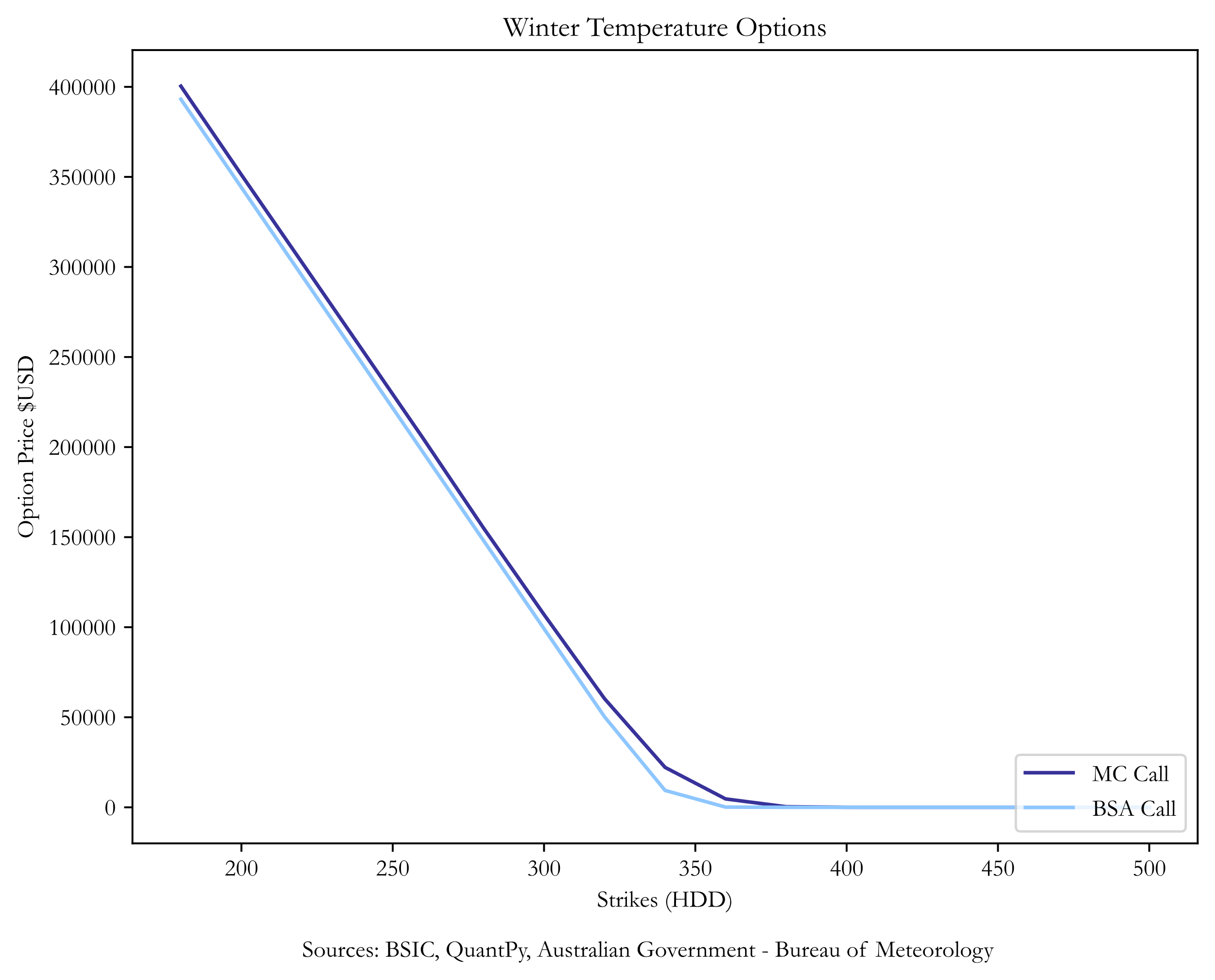
In general, using the Black Scholes approach makes sense because usually during winter periods, the average temperature does not often exceed the reference temperature (18 degrees C), at least not in European countries and in the US. However, Sidney’s temperature presents a lot of upper outliers. Specifically, when simulating the Sidney temperature data over the upcoming winter months using the Monte Carlo model from the previous section, the probability that the average temperature is higher than the reference point varies between 3.3% and 7.6%. This influences the price of the option as the Black-Scholes approach incorporates a term related to the cumulative distribution function of the temperature. The price of a winter call option estimated by our risk-pricing model, expiring on the 31^st of August, is $99,162.

On another note, the Monte Carlo valuation computes the discounted expectation of the payoff under the risk-neutral probability measure, by simulating the temperatures and then calculating the number of resulting heating degree days in the valuation period. We will use the fundamental theorem of asset pricing, which states that:

$\frac{C_t}{B_t}=E_Q\left[\left.\frac{C_t}{B_t} \right\rvert\, F_t\right]$

where $C_t$ represents the payoff, $B_t$ represent the bank account based on the risk-free rate, $E_Q$ represents the expectation under the risk-neutral probability and the conditional $F_t$ is the representation of the information available to market participants up to time t. Considering the call option payoff equal to $\alpha * \max (D D-K, 0)$ :

$C_t=B_t * E_Q\left[\alpha * \max (D D-K, 0) \mid F_t\right]$

For $\mathrm{M}$ simulations, the final payoff of the call option is equal to:

$C_t=e^{-r \tau} * \frac{1}{M} * \sum_{m=1}^M\left[\alpha * \max \left(D D_m-K, 0\right)\right]$

The price of a winter call option expiring on the 31^st of August, using the Monte Carlo approximation, is equal to $106,958.

To conclude, we provide a plot of call option prices for different strikes to showcase that the Black-Scholes method is quite similar to the Monte Carlo valuation. However, the latter is more suitable for pricing Australian temperature options, and the choice between the two should be rigorously researched when pricing these derivatives in other geographical areas.

References

[1] Weather Derivatives Tutorial, QuantPy

[2] Financial Management of Weather Risk, MPRA Paper No. 35037

[3] On Modelling and Pricing Weather Derivatives, Fat Tails Financial Analysis AB, Department of Mathematics, KTH

[4] Weather Derivatives: Pricing and Risk Management Applications, Institute of Actuaries of Australia

[5] Weather Derivatives and the Market Price of Risk, Journal of Stochastic Analysis

Published by BSIC on 3 March 20243 March 2024

0 Comments

Leave a Reply Cancel reply

Corporate Finance Markets

Exploring the Practicality of Merger Arbitragе

Markets

Market Recap 05/05/2024

Markets

A Systematic Approach to Credit Investing

A Practical Guide to Pricing Weather Derivatives

Published by BSIC on 3 March 20243 March 2024

0 Comments

Leave a Reply Cancel reply

Related Posts

Corporate Finance Markets

Exploring the Practicality of Merger Arbitragе

Markets

Market Recap 05/05/2024

Markets

A Systematic Approach to Credit Investing