Introduction
Interest rate derivatives (IRD) represent the largest segment of the OTC derivative market. As of June 2023, the global OTC derivatives notional outstanding amounted to $714.7tn as reported by the Bank for International Settlements (BIS). The biggest share of this market is represented by IRD and FX derivatives, with notional outstanding of respectively of $573.7tn and $120.3tn. IRD market can be further dissected into the sub-markets for interest rate swaps ($465.9tn), forward rate agreements ($61.8tn), and options ($45.8tn).
IRDs are more challenging to evaluate than equity and FX derivatives. First, the behaviour of interest rates is far more complicated, requiring a model to describe the stochastic process that interest rates follow. A second issue is that interest rates are used both in computing the payoffs of such derivatives, and for discounting purposes.
In this article we provide an overview of the main fixed income options, by presenting their main features, how they can be used to hedge interest rate risk, and by briefly touching upon some issues related to the assumptions underlying their valuation models. In the final section, we present a practical example on how to use Black’s formula to extract the Implied Volatility of Caplets, using Python.
Black’s Model
The Black formula was originally designed to price options on commodity futures (Black 1976), due to its robustness, simplicity, and the precision it offers, it is widely adopted by traders to quote prices of interest rate derivatives, from caps and floors to swaptions.
Important for our discussion is the concept of numeraire. A numeraire is the unit of account used to express the value of a financial security. Numeraires are useful for pricing because it can be shown (Harrison and Kreps) that relative prices (ratio of an asset to a numeraire) are Martingales under risk-adjusted probabilities. That is, there exists a probability measure  such that the relative price is a Martingale:

This allows us to price the asset at time  , since:

Numeraires can be any asset that has a strictly positive value and is self-financing. For the sake of the article, one numeraire important for us is the time  price of a zero-coupon bond
  that pays $1 at time
  (assuming no default risk) and let the value at time of a generic derivative expiring at be
  . We can rewrite the normalized price of the derivative as:


It can be proven that in the world defined by numeraire  it holds:
![\widetilde{s}\left(t,T\right)=E^{\mathbb{Q}^T}\left[\widetilde{s}\left(T,T\right)\right]=E^{\mathbb{Q}^T}\left[\frac{s\left(T,T\right)}{Z\left(T,T\right)}\right]=E^{\mathbb{Q}^T}\left[s\left(T,T\right)\right]](https://bsic.it/wp-content/ql-cache/quicklatex.com-545a00de78c75c0551a4f4f4813284e1_l3.png "Rendered by QuickLaTeX.com")
Where ![E^{\mathbb{Q}^T} [\cdot]](https://bsic.it/wp-content/ql-cache/quicklatex.com-6804aee25be17d58fd7c3f43a637bf97_l3.png "Rendered by QuickLaTeX.com") represent the expectation under T-forward measure, and
represent the expectation under T-forward measure, and  .
.
Consequently, the price of the derivative security at time is given by:
![s(t,T)=Z(t,T) E^{\mathbb{Q}^T} [s(T,T)]](https://bsic.it/wp-content/ql-cache/quicklatex.com-5c7eacc4da191a190df6555f8cfe3918_l3.png "Rendered by QuickLaTeX.com")
The reason why it is called “forward” measure stems from an important result regarding forward prices. Let’s consider a forward contract at time for the delivery of a generic asset  at time . From the previous equation, the value is given by:
![f(t,T)=Z(t,T) E^{\mathbb{Q}^T} [F(t,T)-\theta(T)]](https://bsic.it/wp-content/ql-cache/quicklatex.com-d676e785e97473b90fadf3c80ba4c4f4_l3.png "Rendered by QuickLaTeX.com")
where  is the forward price determined at time , such that the value at inception is equal to zero. It follows that:
![Z(t,T) E^{\mathbb{Q}^T } [F(t,T)-\theta(T)]=0](https://bsic.it/wp-content/ql-cache/quicklatex.com-5945535b4244fcd67908ac4bb7d60b00_l3.png "Rendered by QuickLaTeX.com")
Or
![F(t,T)=E^{\mathbb{Q}^T} [\theta(T)]](https://bsic.it/wp-content/ql-cache/quicklatex.com-9c827081cdfdeaef3f299ebb22df6552_l3.png "Rendered by QuickLaTeX.com")
Given the convergence property of forward price  we have that:
![F(t,T)=E^{\mathbb{Q}^T } [F(T,T)]](https://bsic.it/wp-content/ql-cache/quicklatex.com-8c7eaaed660bee03f4b85e208aa45b0a_l3.png "Rendered by QuickLaTeX.com")
In other words, under the T-forward measure, the forward price for delivery at time is a martingale, and its process can be described as a driftless log-normal diffusion process:

where  is the diffusion term of the forward price.
In the world defined by numeraire  , the price at
  of a European call option with strike price
  , with expiration on the forward price
  , which has constant volatility
  , is given by:
![c(0,T)=Z(0,T) E^{\mathbb{Q}^T } [(F(T,T)-K)^+ ]](https://bsic.it/wp-content/ql-cache/quicklatex.com-fd266e50176c0753e7890e1414d84eef_l3.png "Rendered by QuickLaTeX.com")
where it can be proven that:
![E^(\mathbb{Q}^T ) [(F(T,T)-K)^+ ]=E^(\mathbb{Q}^T ) [F(T,T)]N(d_1 )-KN(d_2 )=F(0,T)N(d_1 )-KN(d_2 )](https://bsic.it/wp-content/ql-cache/quicklatex.com-9d0761e476692566fba0c04fb7d3a8d7_l3.png "Rendered by QuickLaTeX.com")
where:
![d_{1,2}=\frac{ln\left[\frac{F(0,T)}{K}\right]\pm\frac{\sigma_F^2}{2} T}{σ_F \sqrt{T}}](https://bsic.it/wp-content/ql-cache/quicklatex.com-1a314f3389df8dfb443a72f88eb870c7_l3.png "Rendered by QuickLaTeX.com")
Therefore, the value of such call option is given by:
![c(0,T)=Z(0,T)[F(0,T)N(d_1 )-KN(d_2 )]](https://bsic.it/wp-content/ql-cache/quicklatex.com-f34610208890766e0146736e9fc22f83_l3.png "Rendered by QuickLaTeX.com")
Similarly, the price of a European put option is:
![p(0,T)=Z (0,T) [KN(-d_2)-F (0,T)N (-d_1)]](https://bsic.it/wp-content/ql-cache/quicklatex.com-10ae099f49d92469bfc23d61971a7acc_l3.png "Rendered by QuickLaTeX.com")
Bond Options
Bond options work like their equity peers, they give the right to buy/sell a certain bond, at a certain strike price, by a particular date. Usually, bond options are issued together with bonds, giving rise to instruments such as callable bonds and puttable bonds.
Callable bonds give issuers the right, but not the obligation, to repurchase the bond before its maturity date, typically at a premium. Why do institutions issue callable bonds? A popular explanation is the “hedging interest rate risk” theory, in which callable bonds allow firms to refund at lower interest rates. Several argue that “indifference should obtain”, since the call feature is exactly offset by the higher yield that bondholders require. Callable bonds might allow an issuing firm to deal with the “debt overhang problem”. A firm (acting in the interest of shareholders) might not invest in projects with positive NPV because part of the benefits from the new projects would go to existing bondholders, and one way to solve this is to allow firms to call back outstanding debt. An alternative role for callable debt would be a signalling mechanism. Under asymmetric information about the firms, insiders might know more about the firm than outsiders. If outsiders can’t infer quality, callable debt might be useful as means of signalling.
Puttable bonds instead come with an embedded put option that grants the buyer the right to sell the bond back to the issuer at a predetermined price before maturity. This mechanism offers investors protection against rising interest rates, enabling them to exit their investment and potentially reinvest in higher-yielding opportunities.
How can we value such instruments? The key is to see them as portfolios of a unit of the non-callable/non-puttable bond combined with a position in the option.
A callable bond is equivalent to a long position in the underlying bond  combined with a short position on the European call
  , and all else equal a callable should have higher yield than a non-callable. The call option can be valued using Black formula:
![c\left(0,T\right)=Z\left(0,T\right)\left[B^{fwd}\left(0,T\right)N\left(d_1\right)-KN\left(d_2\right)\right]](https://bsic.it/wp-content/ql-cache/quicklatex.com-7c7504f80c8aa321eb5299ca7797b180_l3.png "Rendered by QuickLaTeX.com")
Whereas a puttable bond is equivalent to a non-puttable bond plus a put option. In this case since the buyer has the benefit of having a limited downside, he/she requires a lower yield than a non-puttable bond. Assuming the put is European, the pricing formula for the put option is:
![p\left(0,T\right)=Z\left(0,T\right)\left[KN\left(-d_2\right)-B^{fwd}(0,T)N\left(-d_1\right)\right]](https://bsic.it/wp-content/ql-cache/quicklatex.com-e97af03435e20ae9a2ab7ca442d10e96_l3.png "Rendered by QuickLaTeX.com")
Please note that  is the forward bond price, with volatility
  , which can be calculated using formula for forward prices with known income:

where  represents the present value of the coupons that will be paid out to bondholders during the life of the option.
Caps & Floors
An interest rate cap is a portfolio of caplets, where each caplet is a call option on interest rates. Conceptually a cap works exactly like an IRS, except that in the case of a cap, the holder has the optionality to proceed with the swap (paying fixed) and reach reset date only if it yields a positive payoff, i.e., when interest rates are higher than the strike rate. Consider a single caplet maturing at time  , with strike
  , and define
  , or
, or  , where
  is the annual frequency of payments. The payoff (at ) of the caplet is:
![N\ \delta\left[r\left(T_i,T_{i+1}\right)-r_K\right]^+](https://bsic.it/wp-content/ql-cache/quicklatex.com-45f498d4642051c8292afa29a88ece9f_l3.png "Rendered by QuickLaTeX.com")
where  is the notional amount,
  is the reference floating rate, with reset date . Since at expiration we have that the reference floating rate is equal to the forward rate
  with volatility
  (which is a Martingale under the T-forward measure):
![N\ \delta\left[f\left(T_i, T_i,T_{i+1}\right)-r_K\right]^+](https://bsic.it/wp-content/ql-cache/quicklatex.com-a9993dff58bc7c1586b9dd12a87703f1_l3.png "Rendered by QuickLaTeX.com")
Using the Black formula (industry standard) we can value the caplet maturing at :
![Caplet\left(0,T_{i+1}\right)=N \delta Z\left(0,T_{i+1}\right)\ \left[f\left(0,T_i,T_{i+1}\right)N\left(d_1\right)-r_K N\left(d_2\right)\right]](https://bsic.it/wp-content/ql-cache/quicklatex.com-6f9b2f647014b13fe0f5aee7654d36cf_l3.png "Rendered by QuickLaTeX.com")
where:
![d_{1,2}=\frac{ln\left[\frac{f\left(0,T_i,T_{i+1}\right)}{K}\right]\pm\frac{\sigma_f^2}{2}T}{\sigma_f\sqrt T}](https://bsic.it/wp-content/ql-cache/quicklatex.com-13787a4685e1946a886b369034d2dc42_l3.png "Rendered by QuickLaTeX.com")
Whereas an interest rate floor is a portfolio of floorlets, that is a collection of put options on interest rates, with payoff equal to:
![N \delta\left[r_K-r\left(T_i,T_{i+1}\right)\right]^+](https://bsic.it/wp-content/ql-cache/quicklatex.com-810f44b7fde4381c8339bc6c3d5642a3_l3.png "Rendered by QuickLaTeX.com")
and the Black formula for a single floorlet maturing at is:
![Floorlet\left(0,T_{i+1}\right)=N \delta Z\left(0,T_{i+1}\right)\ \left[r_K N\left(-d_2\right)-f\left(0,T_i,T_{i+1}\right)N\left(-d_1\right)\right]](https://bsic.it/wp-content/ql-cache/quicklatex.com-7dd8e7188cd15bbeed2faf4fda27c064_l3.png "Rendered by QuickLaTeX.com")
The benefit of buying a cap (floor) is to be protected in each period from upside (downside) movements in interest rates. However, if you want to keep the floating interest rate between two desired levels, it is possible to achieve this by constructing an interest rate collar by combining a long position in a cap and a short position in a floor. Collars help in risk management of certain position by establishing a maximum interest rate the borrower will pay, but at the same time agreeing to pay a minimum rate.

Put-Call Parity for Caps & Floors
There exists an equivalent version of put-call parity in the case of caps and floors. Let’s consider a long position in a cap combined with a short position in a floor. We know that the payoff is ![N\ \delta\left[r\left(T_i,T_{i+1}\right)-r_K\right]](https://bsic.it/wp-content/ql-cache/quicklatex.com-8506a2f7fb2675f4145c801b798ebe9c_l3.png "Rendered by QuickLaTeX.com") whenever the interest rate is higher than the strike, while the position also pays the same amount if rates are lower than the strike, i.e., the payoff is the same regardless of the level of interest rates. This is the same payoff structure as a swap (fixed payer, swap rate ); therefore, it follows that:
whenever the interest rate is higher than the strike, while the position also pays the same amount if rates are lower than the strike, i.e., the payoff is the same regardless of the level of interest rates. This is the same payoff structure as a swap (fixed payer, swap rate ); therefore, it follows that:

Flat vs Forward Volatilities
When dealing with caps & floors, volatility can have two different meanings for market practitioners. We may refer to flat volatility or par volatility which is defined as the quoted volatility such that if we use this value inside the Black formula to price each caplet belonging to a cap, we obtain the price at which the cap is trading at. That is, we use the same volatility to value every single caplet, disregarding the fact that their maturities differ, and this can be interpreted as an “average” volatility of the set of individual caplet volatilities.
But if we were to use flat volatilities to price single (equivalent) caplets coming from different caps, we may find that the prices differ, hence erroneously thinking that we have found an arbitrage. Instead, we should use the no arbitrage volatility, referred to as forward volatility, which is the volatility  that characterizes a particular caplet with maturity , independently of which cap the caplet belongs to. Forward volatilities are generally not quoted, and they have to be extracted via a bootstrapping procedure using quoted flat volatilities, after which it is possible to construct the forward volatility curve.
The forward volatility curve may have different shapes, the most common is the hump shape. The shape of the curve varies over time, as the implied forward volatility represent an insurance premium that market participants are willing to pay/receive, such figure increases when uncertainty of future interest rates is higher. It is worth to note that forward volatilities for longer horizons tend to be low due to the mean reverting nature of interest rates.
Refer to the last section of the article for a practical example of how to extract Forward Implied Volatilities from caplets.
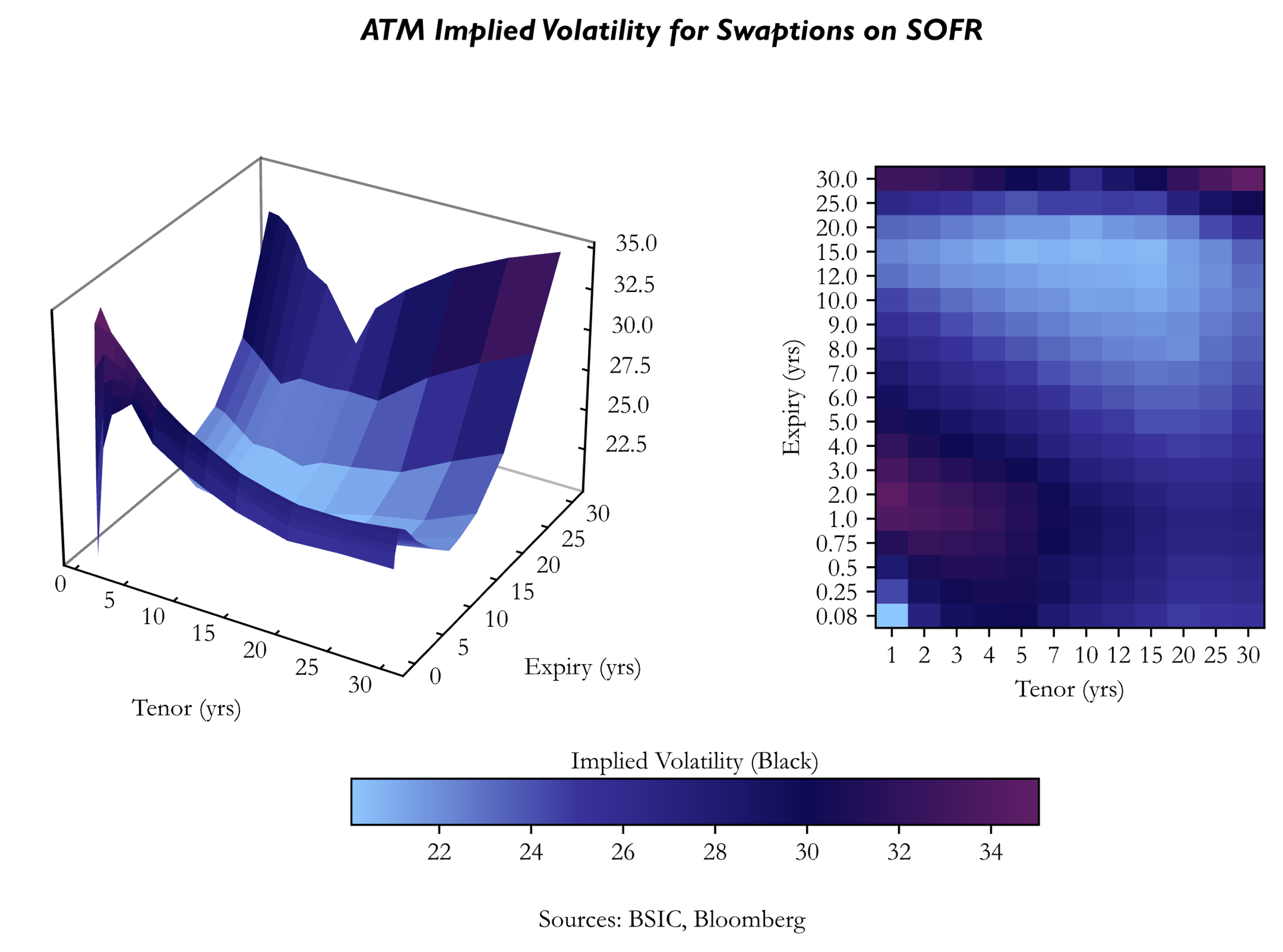
Swaptions
Swaptions are options to enter into a swap, as either fixed rate payers – payer swaption – or fixed rate receiver – receiver swaption. Swaptions can be for example used by companies who want to transform a future floating rate liability (e.g., a loan) to a fixed one. In such case, with a swaption the company can guarantee that the fixed rate of interest they will pay will not exceed a strike rate and they represent a more flexible alternative to forward starting swaps.
Let’s consider a payer swaption, the payoff at maturity is:
![N\delta\left[\sum_{i=1}^{n}Z(T_M,T_i ) \right] [s(T_M,T_n )-r_K ]^+](https://bsic.it/wp-content/ql-cache/quicklatex.com-ef1b7e3e8017e6ff97d0de86ecbbda8d_l3.png "Rendered by QuickLaTeX.com")
where is the notional,  is the future swap rate of a swap underlying the option, starting at
  (maturity of the swaption) maturing at
  , such that at inception the value of the swap is zero.
To understand in a more intuitive way the formula, we can see that the holder of the payer swaption will exercise if he/she can pay the lower rate instead of the market swap rate  . Then, at every payment date of the underlying swap, the holder will gain the constant spread
  , therefore the total payoff from the exercise of the swaption is equal to the present value of each of these gains.
Instead, a receiver swaption the payoff at maturity is:
![N\delta\left[\sum_{i=1}^{n}Z(T_M,T_i ) \right] [r_K-s(T_M,T_n )]^+](https://bsic.it/wp-content/ql-cache/quicklatex.com-ce69cdcab2ca6a37710b917cab9c2c6c_l3.png "Rendered by QuickLaTeX.com")
To value a European payer swaption we use the Black formula, where we assume that the underlying swap rate  at the maturity is log-normally distributed:
![Swpn_K^{pay} (0,T_M )=N\delta\left[\sum_{i=1}^nZ(0,T_i ) \right][s(0,T_M,T_n )N(d_1 )-r_K N(d_2 )]](https://bsic.it/wp-content/ql-cache/quicklatex.com-67ab93008b845efef7bd2093478f305c_l3.png "Rendered by QuickLaTeX.com")
where  is the forward swap rate at time 0 to enter at into a swap with maturity , and
![d_{1,2}=\frac{ln\left[\frac{s(0,T_M,T_n) }{r_K}\right ]\pm\frac{\sigma_s^2}{2} T}{\sigma_s \sqrt{T}}](https://bsic.it/wp-content/ql-cache/quicklatex.com-9e86069aa5ef2316cc49aa449af58177_l3.png "Rendered by QuickLaTeX.com")
With  representing the percentage volatility of the forward swap rate.
Similarly, the time 0 value of a European receiver swaption is given by:
![Swpn_K^{rec}(0,T_M )= N\delta\left[\sum_{i=1}^nZ(0,T_i ) \right] [r_K N(-d_2 )-s(0,T_M,T_n )N(-d_1 )]](https://bsic.it/wp-content/ql-cache/quicklatex.com-8535046b30370d1471f19fcc12af7809_l3.png "Rendered by QuickLaTeX.com")
To our most curious readers, note that in the pricing formulae for swaptions have a different form compared to the ones for bond options, caplets and floorlets. When dealing with caplets for example, forward rates are Martingales when considering a zero-coupon bond as numeraire. In the case of swaptions we have forward swap rates, which can be shown to be Martingales, however under a different equivalent martingale measure (EMM), which is the one associated with the annuity factor ![\delta[\sum_{i=1}^n Z(0,T_i)]](https://bsic.it/wp-content/ql-cache/quicklatex.com-1c85b76a790e2d23680884d5b5c722ca_l3.png "Rendered by QuickLaTeX.com") as a numeraire, called swap measure. In other words, under the swap measure, the expected future swap rate is the current forward swap rate.
as a numeraire, called swap measure. In other words, under the swap measure, the expected future swap rate is the current forward swap rate.
Similarly to caps and floors, there exist a relationship between receiver and payer swaptions:

where  is the value of the forward IRS paying .
Just like caps and floors, swaptions dealers quote the instruments in terms of implied volatilities, that is the volatility which if inserted into the Black formula gives the current price of the swaption.
Beyond Black’s Model
The Black-76 model although being widely used by practitioners when it comes to pricing caps, floors and swaptions, it has two fundamental issues: volatility skew/smile, and negative rates.
In the standard model used for pricing fixed income options the volatility of forward rate  is independent of the strike and maturity, i.e., constant. Nevertheless, this is far from the truth, as implied volatilities exhibit a (1) term structure, and for a specific expiration date implied volatilities display a (2) skew.
In order to more accurately value and risk manage portfolio of options some improvements of Black’s model are needed. An improvement can be done by adopting “local volatility models”. What this class of models does is to search a volatility function  such that the price predicted by the model matches the market for each strike level. In other words, a local volatility model has to “fit the skew”. Nevertheless, such models still fail to accurately reflect market dynamics, and attempts were made to move beyond local volatility with (i) stochastic volatility models, such as the SABR model (Hagan et al., 2002); and (ii) jump diffusion models.
Another issue with the Black-76 model are negative rates, which have been used by several central banks as an unorthodox monetary policy tool to combat persistently difficult economic conditions. The problem is that the model assumes forward interest rate (or swap rate) to be log-normally distributed, which means that it does not support negative rates. A possible solution is to use a shifted log-normal model (also known as displaced diffusion model), where basically the forward interest rate plus a spread () is assumed to be log-normally distributed, so that negative values below the shift are not admissible. The SABR model can also be adjusted in a similar way, resulting in the shifted SABR model. Another alternative which is easy to implement is the Bachelier normal model, leading to have a normally distributed interest rate, although allowing for (with small probability) extreme negative values.
A Practical Application: pricing a strip of Caplets and extracting IVs using Python
In this section, we implement and use Black’s Formula to extract the Implied Volatilities of Caplets from the 6Mx10Y Cap on 6M Euribor with strike  and notional
  , which we mentioned in the section on Caps and Floors. Data and calculations are as of Feb 17, 2024.
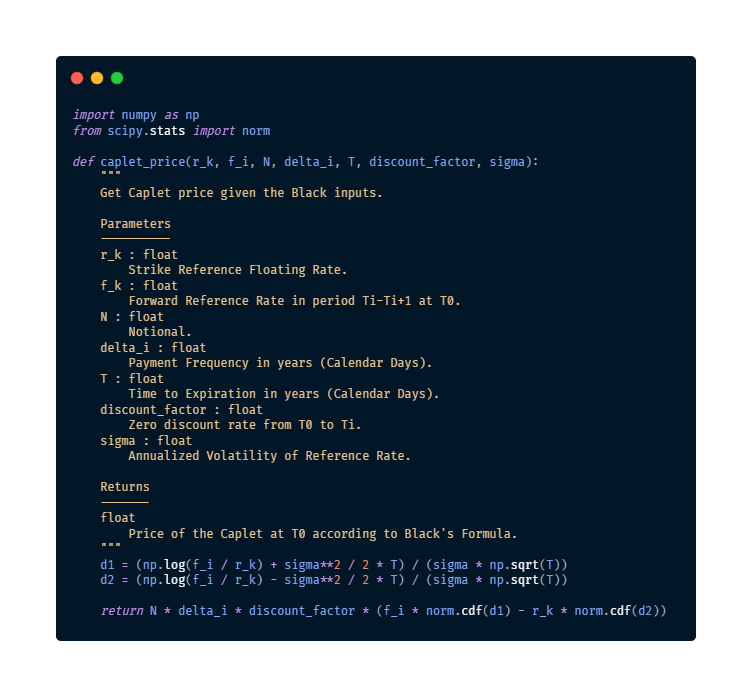
First, we define the function caplet_price, which returns the price of a caplet given the inputs required by Black’s formula.
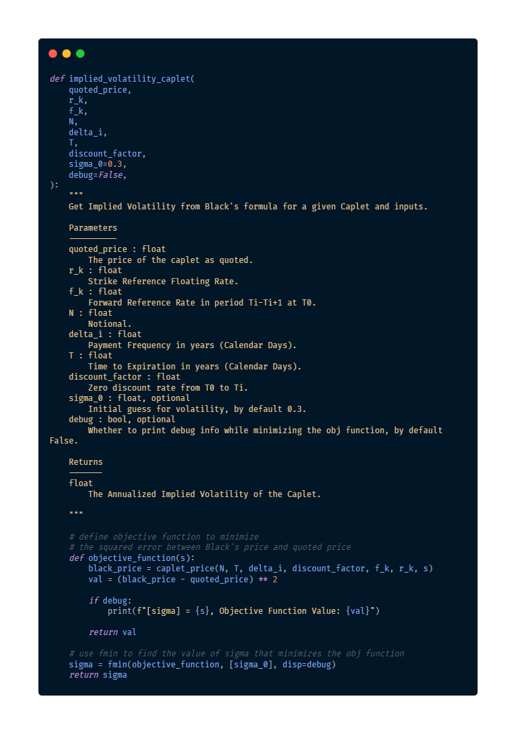
Next, we create a function, implied_volatility_caplet, which, given the quoted price of the caplet, returns the Implied Volatility which, inserted in Black’s formula, returns the quoted price. As there is not a closed-form solution for in Black’s model, we use an iterative procedure which, starting from an initial guess  , finds
  which minimizes the square of the difference between the quoted and Black’s price.
Now that we have defined these two functions, we can proceed to find the Implied Volatility using the data on the caplets composing the cap. Note that  indicates the number of days from the expiration date to the payment and must, as , be converted in years (divide by 365) when plugging into Black’s formula. The Forward Zero Rate is the forward 6M Euribor (from to
  , which corresponds to 6M in this case, since the cap pays semi-annually) at time
  , which is calculated by interpolating the Euribor zero curve and can be found on Bloomberg. The discount factor is the 6M Euribor from to and can also be calculated and found in the same manner. Also recall from earlier the other inputs which will be plugged in Black’s formula: , .
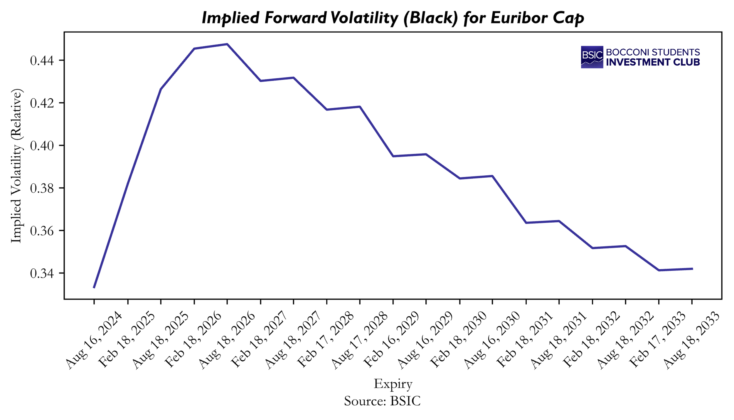
We now iterate through the different caplets and, using the functions defined above, extract the Implied Volatilities for each caplet. The code for this section can be found on this GitHub repository. Below, we plot the IVs found, which present the usual “hump”.
If we compare the Implied Volatilities found through this method and the ones reported from Bloomberg, we might wonder why they differ. Actually, the IVs quoted in the previous section assumed a Normal Distribution of the Reference rate, thus expressing the Implied Volatility in absolute terms (bps), while the Black Model assumes a log-normal distribution, expressing the Implied Volatilities in relative terms. An approximate relationship (Hagan et al, 2002) between normal volatility and log-normal (Black volatility) is given by:

Using this formula, we can see Black and Normal Implied Volatilities are similar, although not equal since, again, the formula just provides an approximation.
References
[1] Darbyshire J. H. M., “Pricing and trading Interest Rate Derivatives”, 2022.
[2] Dieckmann S., “FNCE 2250/7250 Fixed Income Securities – Callable Bonds”, 2023
[3] Hagan P. et al, “Managing Smile Risk”, 2002.
[4] Hull J., “Options, futures, and other derivatives”, 2021.
[5] Lesniewski A., “Interest Rate and Credit Models, 5. Caps, Floors, and Swaptions”, 2019.
[6] Veronesi P., “Fixed Income Securities: Valuation, Risk, and Risk Management”, 2010.
[7] Veronesi P., “Handbook of Fixed-Income Securities”, 2016.


0 Comments