In this article we will skip the introduction of the very fundamental characteristics of ETFs and focus on the more advanced mechanics, here meaning the different replication methods accompanied by a glance at current developments in the respective section. With an understanding of these more advanced mechanics, we will then seek to stress two major weaknesses in the structure of ETFs, secretly exploited by the sponsors and authorized participants. As this is quite a big read, we will provide a quick summary for each topic at the beginning of such, for our rather hasty readers.
For the general structures and basic mechanics of ETFs as well as current regulation and policy issues in the dominant market, the US, we refer the reader to recently published notes of the Congressional Research Service titled ETFs: Issues for Congress (Sep 2018). For a closer look at the current situation in the ETF market we suggest reading our article from March 2019, Investing in the ETF Era, which thoroughly assesses the state of affairs in trading, pricing and risks of ETFs. We also wrote an article on how to implement ETFs in order to enhance the quality of portfolios, from March 2017, Innovation in the ETF Industry: Tales from Quant 2017 Venice, featuring four specific examples of implementation.
Quick update: exchange-traded funds account for $5.2tn of assets globally as of April 2019.
Replication Methods
The discussion of replication methods will be by means of unleveraged long-only ETFs. The most common replication methods are physical and synthetic replication, where physical replication can further be classified into full and sample replication. The use of the respective method generally depends on the tracked indices and, specifically, with regard to the amount of securities comprised in these as well as the underlying securities’ physical appearance on the market and liquidity.
Full Physical Replication
Various methods exist for replicating an index. The most obvious and classic method being physical replication. As the name suggests, this method works by directly buying the underlying securities of the index. The EURO STOXX 50 ETF utilizes this method by investing in the 50 largest companies in the Euro zone and weighing them with the same percentage as the original index does.
The largest concern surrounding ETFs, especially one that’s looked at closely by regulators is their liquidity. The market-making activity that underpins ETFs is fairly prone to failure, as the mechanism relies on authorized participants that buy ETF units at a discount to their underlying assets to then sell them at a premium. The concern arises due to the fact that these participants have no legal obligation to carry out the subject function, hence giving rise to the risk that they may retreat in the event of a market crisis.
Sampling Replication
In short, for large or illiquid indices, the full replication method reaches its limits because it is either impossible or inefficient to buy every security in an index. Such indices are often replicated using the so-called sampling method. With the sampling method, only the most important or liquid securities are purchased because these usually have the greatest influence on the index performance.
In case the choice of the method is an efficiency issue, it can be seen as an optimization problem with a trade-off between the tracking error and cost of replication. Intuitively, for indices of great securities quantity, the increased management effort of periodically balancing larger number of securities comes at higher costs while on the flip side, the larger the sample, the lower the tracking-error. What this means is that the choice of included securities depends on their market cap, as well as criteria related to their sector and fundamentals, generating an optimal basket. This allows the fund to reduce costs by ignoring more illiquid securities with a low index weighting which wouldn’t have a significant impact on the fund. However, the strategy also produces the risk of large tracking errors if a security which is omitted records an exceptional rise.
You would seldomly find the sampling method as a stand alone, but rather used combined with the synthetic method to reduce the potentially high tracking error, this combination is sometimes referred to as the optimization method. One example is the iShares Russell 2000 ETF (IWM B+). IWM invests 90% of its assets in stocks from the underlying index. The assets that remain are then invested in products such a futures, options and swap contracts, as well as in securities not included in the underlying asset. All these are strategically picked by the manager according to what they see the most fit to efficiently replicate the underlying asset. This is especially evident in indices such as the one mentioned earlier, as it allows the management of the fund to not have to buy all the 2000 stocks, and then manage them to match the exact weightings, instead they can match the underlying fund with derivatives only using ~10% of its original assets.
How exactly derivatives contribute to the replication of an index or basket of securities will be discussed in the details of the synthetic method, since the usage of derivative lies at its very core.
Synthetic Replication
In short, exchange-traded funds achieve their investment objectives by either owning the portfolio of securities that is being tracked or relying on derivatives to deliver promised returns. This is done instead of holding the actual basket of goods as is the case with physical ETFs. In the case of replication using derivatives it is referred to as the synthetic method, typically implemented by entering into swap agreements, although, also other derivatives such as futures and options are sometimes used in synthetic funds.
The swap is collateralized with a portfolio of securities to which the ETF has access in case the swap counterparty defaulted on its obligations. It is also key to point out that the securities included in the collateral basket are mostly different than the securities in the benchmark reference of the ETF. Hence, the level of collateralization serves as protection for investors against losses in case the ETF counterparty does not honor the swap contract.
However, Synthetic ETFs haven’t been able to rise to the forefront of the ETF market due to the SEC not allowing any more launches of new synthetic ETFs since 2010 with the only exception of the ban belonging to asset managers who were already sponsoring synthetic ETFs before 2010. Hence, synthetic replication is something mostly seen in Europe. On the continent, the system functions with posted collateral baskets usually composed of securities which come from the swap counterparty’s inventory (typically equities included in well-recognised indices, bonds, cash and funds) that meet the conditions given out by the EU legislation in terms of asset type, liquidity and diversification.
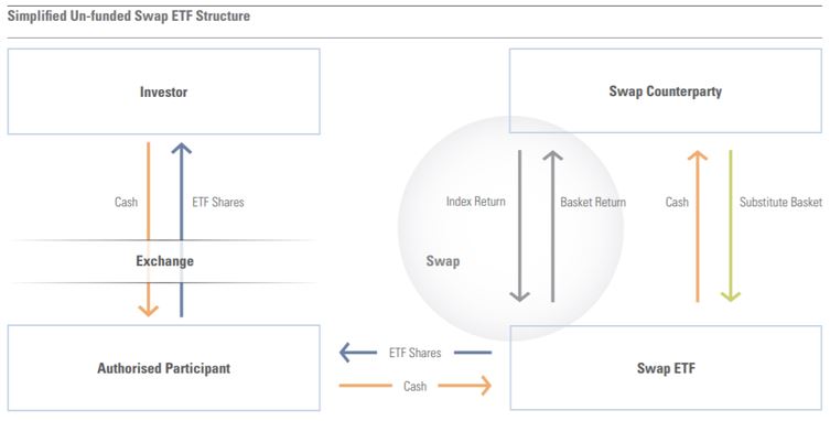
Two main structures exist for synthetic ETFs: unfunded and funded. The unfunded structure relies on the issuer of the ETF creating new shares in exchange for cash from the authorized participant, and then entering a total return swap with a counterparty. A basket of securities is bought with investors’ cash from the swap counterparty by the ETF issuer. The swap counterparty promises the delivery of returns of the reference index, with a swap fee being applied in some cases. In exchange, the return generated by the substitute basket is received by the swap counterparty. The structure benefits ETF issuers as they have ownership of the assets in the substitute basket, and hence are able to liquidate them instantaneously if the swap counterparty defaults.
In the case of a funded swap model/structure, the shares of the ETF are created in the same way, as the issuer transfers the cash received from investors to a swap counterparty. However, the collateral basket is placed into a segregated account with an independent custodian, rather than being owned by the ETF.
To mitigate counterparty risk, UCITS regulations do not allow more than 10% of the fund’s NAV in exposure to a swap counterparty. Hence, the daily NAV of the substitute basket should amount to at least 90% of the ETF’s NAV. This means that at least 90% of the ETF’s NAV prevailing at the time of default is secured for the fund’s holders. The swap is reset whenever the counterparty exposure approaches the 10% UCITS limit (or a lower limit set at the discretion of the ETF provider). In the case of a swap reset, the fund will ask the counterparty to pay the swap mark-to-market by delivering additional securities to top up the substitute basket. Some providers may engage multiple swap counterparties in an effort to minimise exposure to any one of them.
There are several advantages to the synthetic technique. At its core, the method offers a tighter fit with respect to the benchmark as the risk of performance deviation is incurred by the counterparty. Furthermore, the strain of replicating the composition of the index is taken away from the ETF manager as he is guaranteed to receive the index performance through the swap agreement. The flexibility generated by this is a major source of value creation for the fund-cost reduction and liquidity optimization. This advantage are especially prevalent when the costs and risks of physical replication are too high. Another advantage which originates from the swap-based approach is the ability to reproduce indices which would otherwise not be possible to be made into ETFs as they would be too concentrated to abide by diversification requirements set out by the regulators. Lastly, the subject mechanism allows access to certain emerging markets where restrictions are imposed on foreign ownership of local stocks, for example mainland China.
Securities Lending in physical ETFs
In short, with the understanding of replication methods it should be clear that an investor is subject to additional counterparty risk in the case of synthetic ETFs. However, it became more and more common practice by physically-replicated ETFs to also engage in security lending using the underlying portfolio and thus once again exposing its investors to counterparty risk. It is said that securities lending is a fairly simple process that can generate extra returns for ETF investors at low risk and we will assume that the risk-return profile for security lending within physical ETFs is not a reason of concern under normal conditions. Nonetheless, the topic has been raised again now with worries over the quality of collateral that is being used in exchange for the security.
Lending out of the fund’s holdings can actually help increase the products efficiency in tracking an index or other basket of funds since management fees and other costs of the fund are sources of tracking errors. The revenue from security lending is to a large extend used to offset these cost. This is quite evident when considering that empirically 45% to 70% of securities lending fees are returned to the fund, though it is mention worthy that another portion of the fees goes to a lending agent which is usually put in charge of the lending program. Nonetheless, this practice of reducing the total expense ratio is a potential for additional alpha returns to all investors.
On-loan levels vary from fund to fund and in the US funds regulators prohibited to lend more than 50% of its total assets while in the EU there is no regulation for a maximum on-loan yet. Not only it is possible to lend out up to 100% of their portfolio securities but there are some ETFs that even do so.
Knowing the state of securities lending in ETFs, let’s have a look at the problem with the collateral posted against the loan.
The most frequent users of borrowed securities are hedge funds seeking to make profit by selling the security immediately and buying it back when it falls in value. The counterparty risk in the loan is that the short-seller the fund is lending to defaults while owing the security. Luckily, it is common practice for the borrower to provide collateral which should either match or, as often the case, exceed the value of the loaned securities. Therefore, the real risk lies in the possibility that the collateral’s value drops at the same time as the security that the borrower shorted rallies strongly, causing the latter to default on the loan.
As already mentioned at the beginning of the topic, we assume that the additional return outweighs the risks associated with it under normal conditions, which are high quality and quantity of collateral. But concern of investors is that the collateral accepted by ETFs does not fulfil quality requirements for stress situations in the market. One reason of why this concern is raised is that there is a mismatch between the loaned security and collateral; for instance, equity collateral held against government bonds lent. As we have just discussed, the real risk of this practice occurs when collateral and the loaned asset move in opposite direction and it is widely known that government bonds and equity markets have a negative correlation.
Investors have to be careful even when the ETF lists cash as collateral provided by the borrower because it is not unusual that cash collateral is itself reinvested in other assets. Even considering rather low-risk like money market securities, in times of high stress in markets any security can be subject to unexpected extremum.
To conclude, it should be in the hands of the investors whether they want to pursue with the counterparty risk, given full transparency. That, however, is where the rubber meets the road because not all providers of funds disclose all information such as the composition and amount of collateral received, their on-loan levels or counterparty risk mitigation measures. Fundamental research about the fund is important for a solid investment decision.
The Exploitation of ETF Taxation
In short, a “secret” feature which lies in the structure of exchange-traded funds is related to their ability of deferring income taxes on the capital gains they realize. Basically, thanks to a US tax law that dates back to the Nixon presidency, funds are allowed to pay redemptions in kind without any related tax effect. This provision is particularly helpful in the case of ETFs, given the fact that those funds can be traded only through the creation and redemption of ETF shares. Moreover, asset managers and investment banks seem to have been partnering for years to exploit this “tax dodge” by using the so-called “heartbeats”, short-term trades that allow exchange-traded funds to take rid of shares that accrued the greatest capital gains and substitute them with newly acquired stocks, thus avoiding capital-gains taxes.
First of all, in order to understand how this tax deferral mechanism works, it is crucial to have a clear understanding of the ETFs’ distribution process. Investments and divestments in ETF shares are not carried out directly with investors but with banks and investment firms which act as market makers. Transactions between those professional traders and the funds are not settled in cash, they are settled in stocks: an investment in an exchange-traded fund is made by adding to it stocks that are currently included in its portfolio and receiving ETF shares; conversely, a divestment is made by taking stocks out of the fund and redeeming ETF shares. In case of a sale of ETF shares, intermediaries pay cash to investors, tender the shares to the fund and receive back a basket of stocks which will then be sold in the market.
In 1969 the US Congress enacted a law which allows funds to avoid capital-gains taxes in case they pay off investors’ withdrawals using stocks. Specifically, section 852(b)(6) of the Internal Revenue Code states that tax regulation does not apply to a given distribution “if such distribution is in redemption of its stock upon the demand of the shareholder”. Clearly, the above-mentioned rule created a tax advantage to ETF investors with respect to open-end funds investors, since, in the latter, redemptions in kind are more an emergency measure than a standard practice.
The most interesting development that followed the discovery of ETF tax benefits is the creation of “heartbeats”: the asset managers’ way to maximize tax deferrals. A heartbeat trade is a short-term investment made in an exchange-traded fund with the purpose of allowing the fund to allocate shares that accrued a considerable capital gain to the investor, thus avoiding any tax effect. Typically, heartbeats are made by investment banks and have a time horizon of 48 hours.
A simplified example may be useful to understand how an heartbeat trade works. Consider an ETF whose portfolio is composed of five stocks: A, B, C, D and E. Suppose that the fund has to sell stocks A and B because they are no longer included in the tracked index and that the investment in those stocks accrued a sizable capital gain. In order to avoid the capital-gain taxes, the fund asks a bank to make a heartbeat trade and thus the latter invests in the exchange-traded fund by providing it with stocks A, B, C, D and E. Two days later, the bank withdraws its investment and gets paid with the old stocks A and B that the fund was willing to sell. In this way, the ETF does not pay any capital-gain tax related to the redemption and does not register any capital gain on the newly-acquired stocks A and B.
Heartbeats have soon become a standard market practice in the context of exchange-traded funds and even well-known asset managers such as BlackRock, Vanguard and State Street routinely use this technique to avoid capital-gains taxes each time a fund has to change its portfolio allocation.
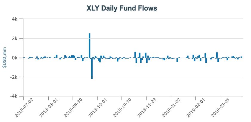
The chart above plots daily flows into the Consumer Discretionary Select Sector SPDR Fund (XLY), an exchange-traded fund managed by State Street that tracks the S&P Consumer Discretionary Select Sector Index. As clearly shown, in September 2018 the ETF received a huge investment of about $2,500mm and only two days later a withdrawal which roughly accounted for the same amount: a classical heartbeat trade. The reason behind the use of such a technique can be easily found in the tracked index’s rebalancing calendar: on the 21th of September 2019 there was a rebalance and the fund exploited the use of heartbeats to defer capital-gain taxes that otherwise it would have had to record on its accounts.
Although heartbeat trades may be seen as unfair and clearly disadvantageous for tax recipients, regulators seem to implicitly approve them and, moreover, the Security and Exchange Commission has recently proposed a rule that would facilitate the use of such trades. Nevertheless, heartbeats are not a way of eliminating taxes; they are able to defer taxes only. When an exchange-traded fund avoids a capital-gain tax, it passes the obligation to the investors, who can in turn defer the tax payment until they sell the ETF.


0 Comments