Alternative approaches to Stochastic Volatility modelling: Part I

Introduction to Stochastic Volatility Models

The distributions of many assets’ price returns tend to show time-varying variance. While returns show little to no persistence in large samples, squared returns exhibit high persistence. Additionally, empirical return distributions tend to show fatter tails than a normal distribution would imply, which supports the idea that their distribution could be modelled as normal, but only conditional to a time-varying volatility parameter. Further, in certain asset return distributions, periods of high (low) volatility tend to be correlated to periods of negative (positive) returns, a phenomenon which is usually referred to as the leverage effect in equities, and more broadly as spot-vol correlation.

A first class of models that attempts to address these issues is that of ARCH/GARCH models. While ARCH/GARCH models describe volatility as a deterministic function of past returns (and/or its past values) the approach in stochastic volatility models relies on describing it as a stochastic variable. The major improvements made to the ARCH model of Engle (1982) and the GARCH of Bollerslev (1986) rely on more complex model forms to incorporate spot-vol correlation, jumps and more generally, to attempt to better describe volatility dynamics. However, these models are highly sensitive to misspecification, particularly when it comes to describing the distribution of their innovations. While the very first versions of these models featured Gaussian innovations, the literature later introduced fatter-tailed innovation distributions to better fit empirical data. Despite these experiments in the GARCH literature, these models describe volatility as deterministic in structure, while their stochastic volatility counterparts still allow for a more flexible specification, where returns and volatility are both stochastic.

The stochastic volatility Model presented by Taylor (1982) models volatility as dependent on a latent variable h called news. The model describes returns $y_t$ as:

$\displaystyle y_t = \beta e^{h_t / 2} \epsilon_t$

$h_t = \mu + \phi (h_{t-1}-\mu) +\sigma_{\eta}\eta_t$

Where $\epsilon_t, \eta_t$ are independent and identically distributed according to a $\displaystyle\mathcal{N}(0, 1)$ . Other extensions of the model feature non-normally distributed, $\epsilon_t$ which we review later in this article. The persistency parameter $\phi$ is assumed to be strictly smaller than 1 for stationarity of the AR(1). Because the parameters $\beta \text{ and } \mu$ have the same effect on $\displaystyle\mathbb{V}(y_t \mid h_t)$ the model is not identified. Scaling $\beta$ or $\mu$ produces the same likelihood. In order to make the model identifiable, a common convention is to set $\beta = 1$ and estimate $\mu$ .

Taking the natural logarithm of $y_t^2$ which we denote by $y_t^* = \text{log}y_t^2$ the observation equation becomes:

$y_t^* = h_t + \text{log}\epsilon_t^2$

Which explains how the news variable $h_t$ influences the squared logarithm of returns. This model can be seen as a discretization of continuous-time models relying on a diffusion process with mean-reverting log volatility.

The problem with the standard formulation of the model lies in the estimation of its parameters $\theta = (\mu, \phi, \sigma_{\eta})$ and of the hidden state path $h_{1:t}$ . The hidden state variable appears nonlinearly, and the distribution of $y_t$ is non-Gaussian, which makes Kalman filtering inapplicable. Other methods like maximum likelihood, the EM algorithm, and direct Bayesian inference are also inapplicable, because the likelihood $p(y_{1:n}|\theta)$ is intractable. We can express the joint likelihood of $y_{1:t}$ and $h_{1:t}$ as:

$p(y_{1:t}, h_{1:t} \mid \theta) = p(h_{1:t} \mid \theta) \prod_{k=1}^{t} p(y_t \mid h_t, \theta)$

And if we were able to derive $p(y_{1:t}, h_{1:t}|\theta)$ we could then integrate over $h_{1:t}$ to derive the marginal likelihood $p(y_{1:t}|\theta)$ as:

$p(y_{1:t} \mid \theta) = \int p(y_{1:t}, h_{1:t} \mid \theta) \, dh_{1:t}$

Since the AR(1) that $h_t$ follows satisfies the Markov property, we could rewrite $p(h_{1:t}|\theta)$ via sequential decomposition as a product of many $p(h_t|h_{t-1}, \theta)$ normal densities, since

$h_t \mid h_{t-1}, \theta \sim \mathcal{N}\!\big(\mu + \phi(h_{t-1} - \mu), \sigma_\eta^2\big)$

We also know that $h_1$ should be distributed according to the stationary distribution of the AR(1), which is normal with mean $\mu$ and variance $\frac{\sigma_{\eta}^2}{(1-\phi)}$ .

The product of these normal densities would be proportional to a multivariate normal density in $h_{1:t}$ since their variables are linearly related.

The challenge comes from the terms $p(y_t|h_t, \theta)$ which are Gaussian, but don’t satisfy the linearity requirement between $y_t$ and $h_t$ , since $y_t | \h_t, \theta \tilde \scriptN(0, e^{h_t})$ .

Hence, we can’t say that the product of the $p(y_t|h_t, \theta)$ terms and $p(h_{1:t}|\theta)$ is proportional to a multivariate normal. This yields an integral with no closed form solution, which does not allow to compute $p(y_{1:t}|\theta)$ exactly.

Parametric modelling

Is there any way to model term $z_t = \text{log}\epsilon_t^2$ that can allow us to implement Kalman filtering techniques? We start with a simple and naïve parametric approach, assuming that $z_t$ follows a Normal distribution with mean and variance equal to the first two moments of the true $\text{log}\chi_1^2$ distribution. In particular, if $\epsilon_t$ is distributed according to a $\scriptN(0,1)$ then $z_t$ is characterized by:

$\displaystyle \mathbb{E}(z_t) = -1.2704$

$\displaystyle \mathbb{V}(z_t) = 4.9348$

Hence, we simply assume $z_t \sim \mathcal{N}(-1.2704, 4.9348)$ becomes linear with gaussian noise, which allows us to apply standard Kalman filtering to estimate the volatility equation parameters $\theta = (\mu, \phi, \sigma_{\eta})$ and filter out the latent volatility process $h_t$ .

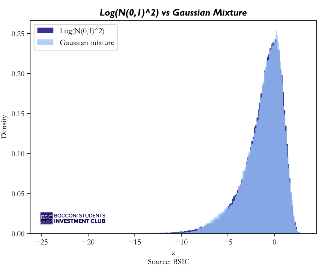
A second and more accurate approach is to approximate $z_t$ with a finite mixture of Gaussian, specifically the 7-component mixture proposed by Kim, Shephard, and Chib (1998). This mixture is designed to closely approximate the true distribution of $z_t = \text{log}\epsilon_t^2$ by matching not only its mean and variance but also its skewness and heavy-tail behavior. Mathematically, we are assuming that the density of $z_t$ is:

$f_{z_t}(z) = \sum_{j=1}^{7} \pi_j \, \mathcal{N}(z \mid \mu_j, \sigma_j^2)$

where the weights, means and variances are fixed constant calibrated by Kim, Shephard, and Chib (1998) to the log-chi-square distribution. To verify how well the 7-component Gaussian mixture reproduces the true distribution of $z_t = \text{log}\epsilon_t^2$ we generated samples from the exact $\text{log}\chi_1^2$ distribution and from the mixture approximation, and run a Kolmogorov–Smirnov (KS) test for equality of distributions. The KS statistic revealed to be extremely small (KS = 0.0039) and the p-value is relatively large (p = 0.094), meaning we cannot reject the null-hypothesis that the two samples come from the same distribution.

The idea behind the Gaussian mixture approximation is that, conditional on the mixture component, the transformed error term $z_t$ is Gaussian. In principle, one could condition on this latent mixture membership and run a separate Kalman update for each component. However, doing so would cause the state distribution of $h_t$ to become a mixture whose number of components grows exponentially over time. To avoid this explosion, we adopt the standard Kim–Shephard–Chib moment-matching approach: after performing the component-wise Kalman updates, we collapse the resulting mixture of Gaussians back into a single Gaussian by matching its first two moments. This preserves computational tractability while retaining the improved tail behavior offered by the mixture approximation.

Simulation study

To assess the performance of the two parametric approximations for the Stochastic Volatility model, we generated synthetic data from known parameters to later check whether the estimates of the models were accurate. Obviously, the returns and volatility processes are generated using Taylor’s stochastic volatility model we described before. Specifically, we simulated 3000 observations with $\mu=0, \phi=0.97, \text{and} \sigma_{\eta}=0.15$ for the latent volatility process, while we considered two different distributions to simulate the returns. In the first case, we stuck to the classical assumption in SV literature and assumed the random shocks $\epsilon_t$ are drawn from a standard Normal distribution. In the second case instead, we drew the random shocks $\epsilon_t$ from a Student-t distribution with seven degrees of freedom, introducing much heavier tails in the returns’ distribution, which is a commonly observed feature in financial markets.

After generating the simulated return and volatility time series with the specified approach, we split the data into training set and testing set. The first 80% of the data is used as estimation sample, where we recover the parameters of the latent volatility process $\theta=(\mu, \phi, \sigma_{\eta})$ using maximum likelihood. The results are presented below:

To summarize, we applied the two methodologies of normal approximation and gaussian-mixture approach on two different series of returns (one with Normal shocks and one with Student-t shocks), so we have 4 different combinations to analyze.

Normal approximation under Normal shocks: this is clearly the best possible case for our naïve approximation because the shocks are actually gaussians; however we still need to remember that the model is misspecified, since we are approximating a log-chi-square distribution with a Normal distribution that simply matches the first two moments, but it cannot fully reproduce skewness and tails of the real distribution. The result is that this approach slightly overshoots the estimation of $\phi$ and then compensates by shrinking the size of volatility parameter $\sigma_{\eta}$ .However, our estimate still seems reasonable.
Normal approximation under Student-t shocks: in this case the model breaks down, because it keeps assuming the shocks in the return series are light-tailed, and the only way it has to explain the empirical heavier tails of the returns is distorting the volatility process. Indeed, it overestimates $\mu$ and $\phi$ , implying a higher and more persistent level of volatility compared to the true value, while in this case it underestimates $\sigma_{\eta}$ .
Mixture approximation under Normal shocks: this is the situation where our model is the closest to being correctly specified, as we are using a distribution for the error term zt which is extremely close to its real one. Indeed, we find that the estimates are satisfying, matching quite closely the true parameters of the underlying latent volatility process.
Mixture approximation under Student-t shocks: in this case the distribution of the error term $z_t$ is again misspecified, because the 7-mixture approach matches a $\text{log}\chi_1^2$ and not a $\text{log}t_7^2$ which is now the real distribution associated with the error term. Hence, the simulated returns have fatter tails than the model assumes, and the only way it can account for the fatter tails is distorting the volatility process. Interestingly, very similarly to the naïve Normal approximation approach, it overestimates $\mu$ , but it behaves differently for the other two parameters. Indeed, it hugely overshoots the estimate for $\sigma_{\eta}$ by doubling it and it compensates by shrinking the volatility persistence parameter $\phi$ .

Finally, with these sample estimates of the latent log-volatility process we can apply Kalman filtering to our simulated $y_t^*$ under Normal and Student-t shocks assumption to extract the filtered estimates of $h_t$ and, more importantly, to generate one-step-ahead volatility forecasts with Taylor’s volatility equation. Thanks to the simulation study, we actually have the “real” volatility process, so we can compare the forecasts on the testing set with the volatility process. Plots for the forecasts are presented and discussed below.

The comparison between the true log-volatility and the models’ forecasts highlights how the two parametric approximations behave under different shocks distributions. A consistent feature of the Normal approximation approach is that its forecasts appear to be systematically smoother than the true volatility path. The Normal approximation often lags behind sudden movements in volatility and underreacts during highly volatile episodes, which makes this naïve approach unsuitable for forecasting purposes.

The mixture approximation approach instead delivers forecasts that are more reactive and better aligned with the true dynamics of the latent volatility process when return shocks are indeed Gaussian. In this case, the mixture is able to correctly approximate the distribution of $z_t$ , allowing the filter to distinguish accurately between noise and genuine volatility changes. However, when returns’ shocks follow a heavy-tailed Student-t distribution, even the mixture approach becomes misspecified. Although it remains more flexible than the Normal approximation, its multiple components still cannot match the extreme tail behavior of a Student-t distribution. The consequence is that the model systematically overestimates future volatility. Under Student-t shocks, the mixture model cannot match the heavier tails and therefore attributes extreme returns to higher latent volatility instead of to fatter-tailed noise. This forces the filter to estimate a volatility process that is too high and too persistent, resulting in overstated volatility forecasts.

Volatility scaling strategies

To assess whether the stochastic volatility model is useful in practice, we apply the Gaussian-mixture approach to daily S&P 500 returns and test its performance in a simple volatility-targeting strategy. We begin by collecting daily price data from 2000 to 2025 and constructing log-returns, which are then split into a training sample (up to the end of 2020) and a testing sample (2021 onwards). The model parameters are estimated only on the training period using the Gaussians mixture approximation for the transformed error term $z_t$ .

Once the parameters of the volatility process are estimated, we run the Kalman filter to obtain the two quantities of interest: the filtered estimate of current log-volatility, and the one-day-ahead forecast of log-volatility. This forecast represents our forward-looking estimate of risk, which we can use to scale our positions in the index.

To evaluate the usefulness of these forecasts, we construct a target-volatility strategy. The idea is to scale the exposure to the S&P 500 such that the portfolio aims to operate at a fixed volatility level. Each day, we compute the leverage required to target a 20% annualized volatility by dividing the target daily volatility by our model’s predicted volatility. For comparison, we construct also a second strategy which uses the naïve 21-day historical volatility as an estimate for next-day volatility. In both cases, the leverage is capped to prevent unrealistic exposures. By applying these leverage adjustments to the next day’s S&P 500 return, we obtain the daily returns of the two target-volatility strategies, and we present below the results.

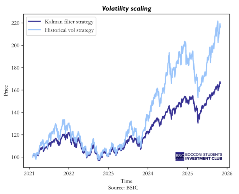
The volatility-scaling experiment highlights a striking difference in how the two strategies manage risk. The strategy based on historical volatility ends up being more exposed throughout the test sample, as it is clear from the steeper growth path. The reason why this happens is actually straightforward after considering the ex-post realized volatility of the two strategies. While the historical-volatility strategy posts a realized volatility of around 21.9%, the stochastic-volatility-based strategy posts a figure closer to 14%, well below the 20% target. In other words, the historical method slightly overshoots the target in our sample by taking on more risk, whereas the SV method undershoots by far the target by being too conservative.

The reason becomes clearer once we connect these empirical results with the simulation findings. In the simulation study, we observed that the Gaussians-mixture approximation approach systematically overestimates volatility when returns are heavy-tailed, as in the Student-t case. The S&P 500 returns share this same characteristic: they display fat tails and occasional large moves that are not well captured by a Normal distribution. As a result, our mixture-of-gaussians model calibrated to match the log-chi-square distribution can explain the fatter tails of the empirical data only by assuming a persistently higher latent-volatility process, which leads to inflated forecasts. Since leverage in our strategies is calculated as target vol / forecasted vol, an overestimated volatility forecast mechanically produces lower exposure to the index.

Taken together, the simulation and the real-data experiment suggest that parametric approximations of the distribution of $z_t$ even flexible ones such as the Gaussians-mixture, struggle when financial returns display pronounced heavy tails. The misspecification propagates directly into incorrect volatility estimates. This highlights a fundamental limitation of parametric treatments of zt and motivates the exploration of non-parametric or semi-parametric alternatives that can adapt more effectively to the empirical distribution of financial returns.

Non-parametric modelling

Given the suboptimal results delivered by standard and variations of the parametric models discussed so far, literature has investigated alternative approaches to the Stochastic Volatility modelling problem. This section will, in particular, discuss the model by Delatona and Griffin [3], giving an overview of the overall structure of the model and some of the benefits it provides. Subsequent work in a Part II will show some practical applications of this model and evaluate its effectiveness on real world data and trading strategies.

From the model in log-linearized form mentioned earlier, Delatola and Griffin start from the following specification:

$\text{log}(y_t^2+c) = h_t +z_t$

$h_t = \mu +\phi(h_{t-1}-\mu) + \sigma_{\eta}\eta_t$

Where the constant $c>0$ is an offset used for datapoints where $y=0$ , for which the natural logarithm is not defined. Unlike normal parametric models, however, (where one would have

$\eta_t, \epsilon_t \tilde \scriptN(0,1)$ Delatona and Griffin suggest the use of a Dirichlet process mixture of normal models, which can be imagined as the nonparametric (i.e., infinite dimensional) extension of this paradigm:

$\displaystyle \lim_{k \to \infty} \sum_{j=1}^{k} p_j \, \mathcal{N}(z \mid \mu_j', \sigma_j^{2})$

$\displaystyle [p_1, \ldots, p_k] \sim \mathrm{Dir}\!\left(\left[\tfrac{M}{k}, \ldots, \tfrac{M}{k}\right]\right)$

With $p_j$ being the mixing components of the different clusters, and the vector $[\mu^', \sigma^'] \tilde H$ being our prior. In such case we find ourselves with a Dirichlet Process, the most classic non-parametric prior in the literature. In this specific instance, however, we will only assume that the mean of the process is cluster specific, while the variance is shared among components. This is because further literature shows there’s little benefit in adding a further layer of flexibility in this instance, giving only higher exposure to potential overfitting and increasing the overall computational complexity of the model [4].

Our model can be hierarchically summarized as follows:

$\displaystyle z_t \mid \mu_t' \sim \mathcal{N}(\mu_t', \alpha \sigma_z^2), \quad t = 1, 2, \ldots, n$

$\displaystyle \mu_t' \sim G, \quad t = 1, 2, \ldots, n$

$\displaystyle G \sim \mathcal{D}(M, H), \quad H \equiv \mathcal{N}(\mu_0, (1 - \alpha)\sigma_z^2)$

With $\mu_0$ being an overall location, $\sigma^2_z$ being an overall variance, $\alpha$ being a smoothness parameter and $M$ being the prior level of confidence in our measure $H$ . To account for zero returns possibly creating issues in the process of fitting the model during MCMC, we can write the unconditional distribution of the log of squared errors as such:

$\displaystyle p(z_t) = W \, \mathcal{N}(\log c, \sigma_0^2) + (1 - W) \sum_{j=1}^{\infty} w_j \, \mathcal{N}(\mu_j', \alpha \sigma_z^2)$

With $W$ being the probability of our returns being exactly 0, which can either be estimated using part of the sample or drawn from a prior, for instance a beta $W \sim Be(\alpha, \beta)$

Within such a framework, the calculations of full conditionals for MCMC techniques are made easier if we express the model as follows:

$y_t^* = h_t^* + z$

$h_{t+1}^* = \phi h_t^* +\sigma_{\eta}\eta_t$

Where $h_t^* := h_t - \mu \quad z_t^* := z_t + \mu \quad h_1^* \sim \mathcal{N}\!\left(0, \frac{\sigma_\eta^2}{(1 - \phi^2)}\right)$

From this, using some algebra, we can obtain good estimates of the moments of t (provided we assume its distribution to be symmetric. Indeed, we have that:

$\displaystyle \mathbb{E}[z_t^*] = \mu + \mathbb{E}[z_t] \approx \mu + \log \mathbb{E}[\epsilon_t^2] - \frac{1}{2}\frac{\mathbb{V}[\epsilon_t^2]}{(\mathbb{E}[\epsilon_t^2])^2}$

$\displaystyle \mathbb{V}[z_t^*] = \mathbb{V}[z_t] \approx \frac{\mathbb{V}[\epsilon_t^2]}{(\mathbb{V}[\epsilon_t])^2} = K(\epsilon_t) + 1$

$\displaystyle e^{\mu}\mathbb{V}[\epsilon_t] \approx e^{\mathbb{E}[z_t^*] + \frac{\mathbb{V}[z_t^*]}{2}}$

However, since many formulas involve infinite sums, we have to use some approximations:

$\displaystyle \mathbb{E}[z_t^*\mid \psi]\approx W\log c+(1-W)\left(\sum_{j=1}^{k}\frac{n_j}{\,n+M\,}\mu'_j+\frac{M}{\,M+n\,}\mu_0\right)$

$\displaystyle \mathbb{V}[z_t^*\mid \psi]=W\!\left((\log c)^2+1\right)+(1-W)\,\frac{\sum_{j=1}^{k}\!\left(n_j(\alpha\sigma_z^2+{\mu'_j}^{\,2})\right)+M(\mu_0^{2}+\sigma_z^{2})}{\,n_{\text{non-zero}}+M\,}$

The estimator of the posterior expectation is the following: $\displaystyle \widehat{\mathbb{E}}[z_t^*\mid y]=\frac{1}{N}\sum_{j=1}^{N}\mathbb{E}[z_t^*\mid \psi^{(j)}]$ with $\psi^{(j)}$ being MCMC samples from the posterior distribution. Similarly,

$\displaystyle \widehat{\mathbb{V}}[z_t^*\mid y]=\frac{1}{N}\sum_{j=1}^{N}\mathbb{V}[z_t^*\mid \psi^{(j)}]+\frac{1}{N-1}\sum_{j=1}^{N}\Big(\mathbb{E}[z_t^*\mid \psi^{(j)}]-\widehat{\mathbb{E}}[z_t^*\mid y]\Big)^{2}$

The overall model can be fitted and updated using an MCMC algorithm with standard techniques like Gibbs samplers and Metropolis-Hasting, and will be discussed in detail, together with the results, in the next part of the article.

Conclusion

This article shows that the practical bottleneck in stochastic volatility (SV) models is not mainly caused by simplicity in model selection, but rather due to the treatment of the transformed error $z_t=\text{log}\epsilon_t^2$

Parametric fixes that make Kalman filtering feasible—either a crude Normal for $z_t$ or Gaussian mixture—work tolerably when returns are close to Gaussian, but they become brittle under heavy tails. In simulation, the Normal approximation smooths and lags volatility; the mixture recovers dynamics well with Normal shocks yet distorts persistence and scale when innovations are Student-t, inflating volatility forecasts. Both outcomes point to misspecification of ztrather than of the latent state equation.

These results motivate stepping beyond fixed parametric forms. A semi-parametric specification for $z_t$ via a Dirichlet process mixture of Gaussians lets the data determine tail thickness, asymmetry, and multi-modality while retaining a standard, stationary AR(1) for log-volatility and enabling tractable MCMC inference. In Part II we will implement this Bayesian nonparametric SV model, detail estimation, and assess whether adaptive modelling of $z_t$ delivers sharper filtering, better one-step-ahead risk forecasts, and more reliable volatility-scaled strategies on real data.

References

[1] Stephen J. Taylor, “Financial Returns Modelled by the Product of Two Stochastic Processes—A Study of Daily Sugar Prices 1961-79”, 1982

[2] Sangjoon Kim, Neil Shephard, Siddhartha Chib, “Stochastic Volatility: Likelihood Inference and Comparison with ARCH Models”, 1998

[3] Delatona E-I., Griffin J.E., “Bayesian Nonparametric Modelling of the Return Distribution with Stochastic Volatility”, 2011

[4] Griffin J.E., “Default priors for density estimation with mixture models”, 2010

Published by BSIC on 23 November 202523 November 2025

0 Comments

Leave a Reply Cancel reply

Market Recap 23/11/2025

The Hidden World of High-Frequency-Trading

Mamdani’s New York: Promises facing Fiscal Reality