An Introduction To Forecasting Growth and Revenues

Projecting growth of earnings and revenues has always been bread and butter of equity analysis, with equity research departments deploying state of art models and tools in order to gain an advantage in forecasting the high growth industries. However, as 2019 certainly has been for many investors a year of growth stocks rallies and downturns, we would like to further explore what is the methodology behind the estimates of revenues and growth, what factors drive their final values and what exactly are the main limitations, in order for an individual investors to better understand risks and sensitivity associated with these commonly taken for granted valuation inputs, in order to in the end discover the limitations concerning the DCF model itself.

Revenue growth vs earnings

The rationale for focusing on the growth of revenues in this article, as opposed to e.g. earnings, comes from two main aspects. First of all, high growth business’ ability to generate revenues is less affected by accounting practices than its reported earnings, which is especially important for quickly growing industries, like tech, pharma or biotech, which tend to have high R&D expenditures and favourable amortization, thus lowering their reported net income. Secondly, even though predicted growth is an important component of value in all valuations, the growth of revenues contributes to a larger portion of value in technology or biotech firms, and almost all of the value in the new technology firms, making it the most critical input in business valuation, which tends to be problematic because of these companies’ typical aspects, that is: low assets, often negative returns, but high expansion potential. Nevertheless, the first part applies to revenues and then we move to earnings, in an attempt to find the potential limitations of both estimates, to which individual investors should pay careful attention.

Basic approaches and methodology

An individual investor looking to input growth rate into his valuation model has got three main quantitative options on how to base hist estimates, which are:

• Historic growth
• Estimating growth from firms’ fundamentals
• Equity research reports

In the first case, historic growth is usually estimated using a basic arithmetic average (AAGR) or geometric average (CAGR) with the main difference being that the latter allows for compounding of growth over time and a smoother growth rate.

Where:

– growth rate in i-th period

– number of period

When it comes to AAGR, even though it allows to determine long-term trends of both revenues or earnings and to suggest an overall direction where the firm is heading, it may not be the best choice when applied to new or fast-growing companies, where it often cannot be an accurate estimate of growth due to short periods available for analysis, as well as the fact that it doesn’t include anything that would account for volatility of the past numbers and simply averages them, meanwhile CAGR smooths out our results as well as diminishes the effect of volatility of periodic growth rates, hence why it seems like a better solution.

With historic growth estimates, however, growth is an exogenous variable, and being input to the valuation models it affects them greatly, while not taking into consideration the structure or operating activities of the company. A solution to this issue may be to make it endogenous, by estimating the growth rate from a firm’s fundamentals. Since the aim of this article is to provide a framework of different methods, we will not go in-depth on accounting principles standing behind this method. In general, there are many scenarios to be analyzed depending whether a firm that is earning a high return on capital and it expects this value to be stable over time or it is earning a positive return on capital that is expected to increase over time, as well as where a firm expects operating margins to change over time, sometimes from negative values to positive levels (1).

In our case though, taking high growth industries as an example, many of these firms report losses while showing large increases in revenues from period to period. The first step in forecasting cash flows is forecasting revenues in future years, usually by forecasting a growth rate in revenues each period. Here we list a couple of remarks concerning these forecasts, listed in A. Damodaran’s The Fundamental Determinants of Growth:

“

1. The rate of growth in revenues will decrease as the firm’s revenues increase. Thus, a ten-fold increase in revenues is entirely feasible for a firm with revenues of $2 million but unlikely for a firm with revenues of $2 billion.
2. Compounded growth rates in revenues over time can seem low, but appearances are deceptive. A compounded growth rate in revenues of 40% over ten years will result in a 40x increase in revenues over the period (1)
3. While growth rates in revenues may be the mechanism that you use to forecast future revenues, you do have to keep track of the dollar revenues to ensure that they are reasonable, given the size of the overall market that the firm operates in. If the projected revenues for a firm ten years out would give it a 90 or 100% share (or greater) of the overall market in a competitive market place, you clearly should reassess the revenue growth rate.
4. Assumptions about revenue growth and operating margins have to be internally consistent. Firms can post higher growth rates in revenues by adopting more aggressive pricing strategies but the higher revenue growth will then be accompanied by lower margins.
5. In coming up with an estimate of revenue growth, you have to make several subjective judgments about the nature of competition, the capacity of the firm that you are valuing to handle the revenue growth and the marketing capabilities of the firm.”

Making that last remark, we arrive at equity research analysts, but before we jump into subjective qualities of growth analysis, let’s first introduce two main approaches when analyzing growth potential, that is – a top-down or a bottom-up approach.

Top-down vs. bottom-up approach

A top-down approach to growth estimation signifies that, rather than analyzing potential growth of a company based on its historical performance, it starts with total market size, potential market growth, market share likely to be attained by the company and then subsequently – growth. In this method all types of methods are used depending on the industry, starting from fairly trivial linear regressions and going as far as complex macroeconomic models that may even incorporate social policy impact on growth rates, as well as weighted probability models of different market growth scenarios for long term predictions.

A Bottom-up approach, on the other hand, uses, amongst other data, the average prices, market share and number of customers in order to estimate business’ revenues and potential for growth. Most public companies provide guidance in their reports on how to estimate their revenues bottom-up, reporting e.g. for a restaurant chain: a store count, same stores sell growth, as well as key drivers of growth including new product launches or capital expenditures. Then analysts may adjust or compare these projections for macroeconomic factors like GDP growth, disposable income or demographic trends, which might be more accurate when analyzing already established, public companies operating in a more stable environment.

However, in the end, the final models differ greatly between the industries and sound understanding of the factors driving the company’s revenues and expenses is crucial. Hence why many ER analysts claim that it’s an art rather than a trivial application of a catch-all formula. From that, we may conclude that it is very difficult for any individual investor to compete with professional analysts and furthermore, that if only appropriate models were built, the necessity of employing analysts in order to build such models would go obsolete.

So can you beat the analysts?

Thus we may assume, that if indeed the analysts have better understanding of the underlying business, they are better informed due to access to high-quality data or bank’s internal databases and that if the firm we are trying to value is followed by a large number of analysts, then our estimates using historic growth or publicly available data cannot surpass the quality of estimates that emerge from the industry analysts. However, is this always the case?

The data is quite clear, as a large number of studies and literature shows that short term estimates prepared by analysts outperform historic growth projections, as the mean relative absolute error, which measures the absolute difference between the actual earnings and the forecast for the next quarter, in percentage terms, is smaller for analyst forecasts than it is for forecasts based upon historical data.

On top of that investors seem to have limited attention and are unable to immediately process all information relevant to future earnings (Sims, 2003; Hong, Torous, and Valkanov, 2007; Cohen and Frazzini, 2008; Hirshleifer, Lim, and Teoh, 2009). In particular, DellaVigna and Pollet (2007) demonstrate that investors have limited attention regarding the longterm earnings implications of information.

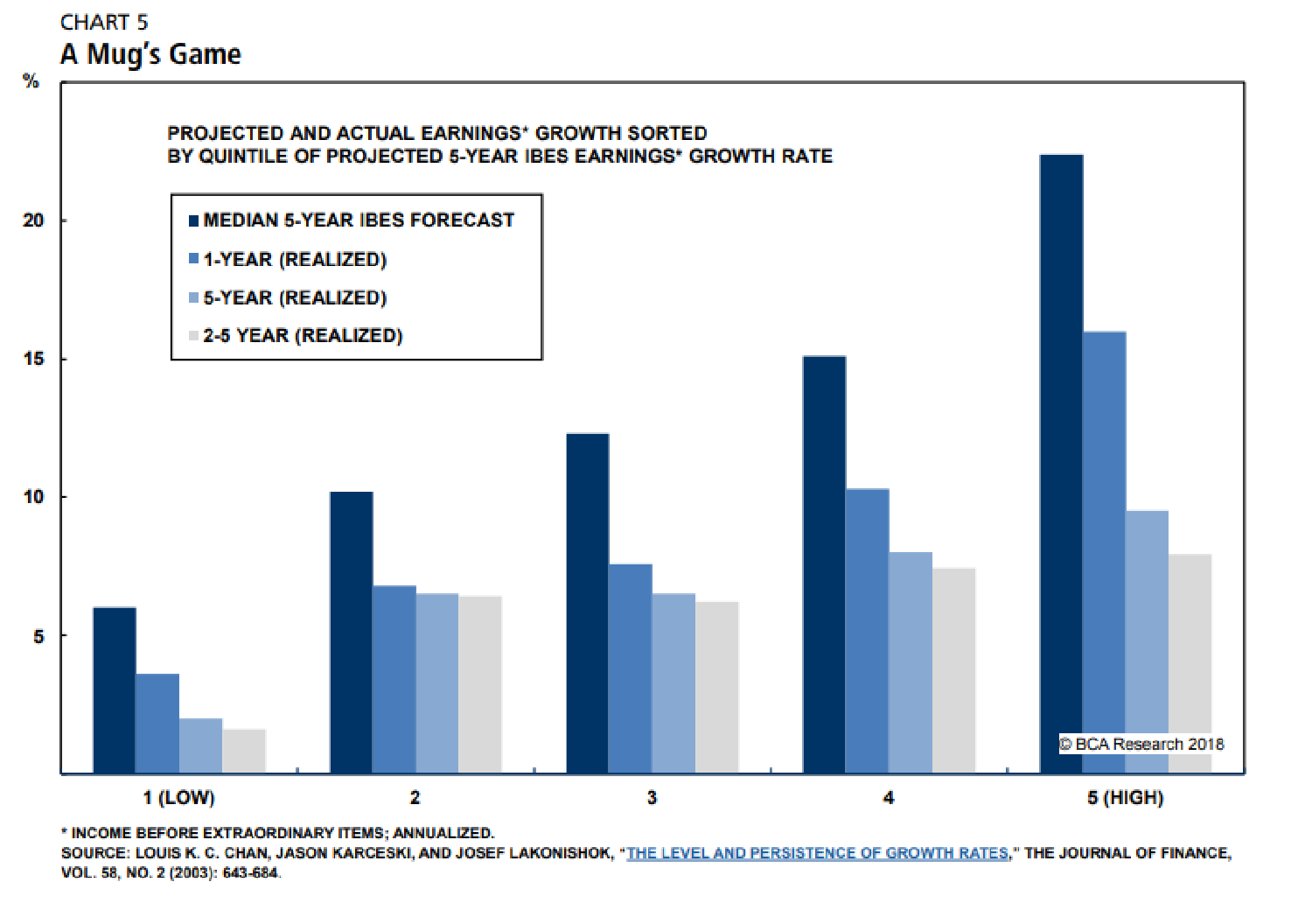
However, there are a couple of remarks to be made, when it comes to analysts’ estimates. As analysts tend to be more accurate than time-series analysis over the periods of 1-2 years, over 5 year periods the analysts’ recommendations prove to carry little accuracy and since technically a long term growth rate period is usually applied to valuation, these estimates should be taken with additional consciousness.

Source: Financial Times

It is worth noting however, that in smaller cap stocks, analysts can “add value” as their estimates show to have bigger carry over, as buy recommendations tend to perform better and affect the price more, than sell recommendations, probably due to smaller amount of data available to investors, when compared with high cap stocks. (2). Quoting legendary value investor Benjamin Graham:

“Because the experts frequently go astray in such forecasts, it is theoretically possible for an investor to benefit greatly by making correct predictions when Wall Street as a whole is making incorrect ones. But that is only theoretical. How many enterprising investors could count on having the acumen or prophetic gift to beat the professional analysts at their favorite game of estimating long-term future earnings?”

Now, having discussed the rationale, methodology and limitations of estimating growth rates, we will discuss the limitations that may be found within the DCF model itself.

Limitations of the DCF models

Discounted Cash Flow (DCF) Analysis is a commonly used valuation method for equity investments. A DCF analysis involves the projection of unlevered free cash flows for a period and then it uses either a terminal value or a terminal growth rate method to demonstrate the future cash flows of the investment. All these future cash flows are discounted using the cost of capital of the firm, generally Weighted Average Cost of Capital (WACC) is the metric used. We argue that there are common pitfalls that these valuation methods might face:

Too Short Forecast Horizons:

Generally, cash flows are projected for a short time horizon like five years.  Due to the view that earnings projections beyond a certain length of time can be highly suspect. However, we don’t see this as a sound way for valuing equities. The median S&P500 PE ratio stands at 14.76, therefore we believe that a long forecast horizon is essential for proper financial valuations as market prices reflect expectations of earnings for many years. The most common solution to compensate for the lack of a long enough cash flow projection is a terminal value that should represent the present value of future earnings when the cash flow projections horizon elapses. However, we see several possible flaws for a terminal value:

• Business cycles do have significant effects on the company’s cash flows and their effects change as time passes. Therefore, a terminal growth rate can be an erroneous way to value future cash flows.
• Some companies lose growth momentum as consumer taste changes and that is hard to quantify issue for financial models.

The long-term growth of economies fluctuates. Therefore, some projections may turn out to be a non-economic terminal growth rate. This effect can be especially strong for Emerging Markets equities as EM economies tend to have a more volatile long-term growth rate. While having volatile long-term growth rates, EM equities tend to be covered less by Equity Research Analysts so the existing research reports and price targets must be reviewed with caution.

Another point to be cautious about is sectors where companies have significant advantages through the patents that they own. These types of sectors include technology and pharma companies that tend to have higher returns from products when they have the exclusive rights over their products, but they tend to lose their margins when patents expire, and products become generic. A better way to project this way can be using a product life cycle model that is valid for patented products and generic product times. However, another thing to consider, even when products are patented, is the release of a similar product that can replicate the patented product.  Too short cash flow projection horizons lack the holistic approach that is needed for these types of sectors as there can be unique developments that lead to breaking points for companies.

The short forecast horizons can also cause errors in the long term cost of capital. The calculation of WACC is dependent on the cost of debt and equity of the firm. However, as interest rates fluctuate frequently that causes the cost of debt for a company to be volatile as well. This trend can be evident when market cycles are at tipping points. For example, nobody would expect current levels of interests for European debtors. This is particularly an issue for both the projection of a company’s financials and the projection of WACC.

As a consequence, we believe that too short forecast horizons cause problems regarding projecting future cash flows and costs of capital. Even if a terminal value is used to forecast beyond the projection horizon terminal values are quite dependent on economic data which tends to be volatile. These effects can be especially important for companies that operate in fragile economies such as emerging markets. Any valuation must be reviewed carefully with a particular focus on how economic developments can affect these valuations.

Diminishing returns on investments 

Another important thing to consider when preparing or reviewing equity valuations arises from an important financial theory: Empirical studies show that on a long enough time horizon a company’s return on investment will converge with its cost of capital due to competitive markets. This theory stands on the common idea of competitive markets, the higher the return on investment of a company is relative to its cost of capital more competitors will try to enter the market and they will squeeze the margins of the business. As a result, projecting terminal values as a sustainably higher value then a company’s cost of capital can turn out being economically wrong. For example, the lucrative cell phone business of Nokia has experienced devastating downward trends in their margins and market shares as smartphones have become more popular. Also, it is important to consider the opposite case: in which companies that leverage innovation and research can increase their returns on investment considerably more than the terminal value projections. This can be particularly common for companies operating in the technology, biotech and pharma industries. A huge success from a patented drug can lead to returns that are quite higher than projections.

Sources:

1. Damodaran A., 2008, Growth and Value: Past growth, predicted growth and fundamental growth, NYU Stern, 2008
2. Smith C., How accurate are sell side analysts, Financial Times Alphaville, November 2018https://ftalphaville.ft.com/2018/11/13/1542091438000/How-accurate-are-sell-side-analysts-/

TAGS: Market Recap