The purpose of this article is to analyse the performance in the European markets – during the last five years – of two strategies that refer to two well-known market anomalies: the value and the size anomalies. Before looking at the results of our research, we will briefly discuss the theory behind them.
A Definition of Financial Anomaly
A financial anomaly is a cross-sectional and time series pattern in portfolio returns that is not predicted by a central model. In the present analysis, the model is represented by the famous CAPM. The CAPM theory, introduced independently by W. Sharpe and other economists in the 60s, develops the work of Markowitz on capital allocation and portfolio theory. It aims to predict the expected return of an investment strategy, based on the expected returns of the market and on the sensitivity of the returns of this strategy to the returns of the market. Briefly, the model assumes that all investors are rational, that is that they prefer the highest possible return for each level of risk. This assumption, together with other minor hypothesis, implies that the market is efficient, because investors either buy or sell securities until their return is the “correct” one. Like in the Markowitz’s model, risk is expressed as the standard deviation of the returns of the strategy. However, since investors can diversify their investment, the part of risk that is rewarded with higher (expected) returns is just the one that cannot be diversified away. This part is reflected by the market Beta, that represents the part of the movement of the stock linked to the movement of the market. The final formula of the CAPM is, finally, as follows:
![]()
Empirical studies, however, have found several examples of anomalies, meaning, again, returns of fixed, predetermined investment strategies not explained by the CAPM. This may be due to two reasons: either that the CAPM does not hold – for instance because there are factors other than the market that explain the returns of a strategy – or else that the CAPM does hold, but the assumption that the market is efficient is simply too strong. This second explanation is for sure valid for some anomalies, since these have naturally disappeared once someone revealed them, simply because investors started to exploit them. Today, we will just go through two anomalies: the value and the size anomalies. These are at the basis, for instance, of the so-called Fama and French three-factor model.
General Overview of Value and Size Anomalies
The value anomaly is probably the oldest to have been investigated in financial markets. It is known since the ‘40s, but has been formally tested only during ‘70s and ‘80s. The key variable is the Book-To-Market ratio, that is, the inverse of the P/BV ratio. According to several analysis, high BtM stocks (“Value stocks”) usually outperform low BtM stocks (“Growth stocks”), even though periods when this tendency is reversed exist. One simple explanation for this anomaly is that value stocks are basically “cheaper” from an accounting standpoint. Another more sophisticated explanation links this ratio to the riskiness of the stock – since usually companies under distress fall into this category – and thus the excess return simply points to the fact that the Beta of the CAPM fails to “highlight” this specific risk. Finally, there exists a behavioural explanation: investors are sometimes fascinated by “glamour” stocks, and tend to overpay for them, thus reducing their future returns (think for instance at the prices of tech companies during the tech bubble).
The size anomaly, instead, has been first analysed in 1981 by Banz, according to whom “small” companies, in terms of market capitalization, systematically outperformed “big” companies. Again, some explanations have been proposed. For instance, some say that this indicator is once more a source of risk: small companies tend to be more volatile than large companies, and the beta may not be a perfect indicator of this risk. Another possible explanation is that stock prices’ growth is linked to the economic growth of the company, and that since for a small company is easier to grow faster, the same may be true for its shares. However, it must be said that the size effect has since them almost disappeared.
Empirical Tests
As hinted at the beginning of this article, our purpose is to test whether these two anomalies have shown up in the European financial markets during the last five years. In order to do so, we used the STOXX Europe 600 index, which contains 600 stocks of small, mid and large companies across 17 countries in the European region. This index is thus a good choice in terms of diversification across geographical markets, capitalization (which is required to compute the size strategy) and business sectors. Its major drawback is that it includes stocks traded in different currencies, and thus some adjustments have to be made, in particular with respect to the market capitalization. The following paragraph explains how we practically performed the tests for the two anomalies.
First of all, we computed monthly (log) returns for each stock starting from January 2012 and ending in January 2017. Then, we created quantiles for each year with respect to the variables of interest (4 for the BtM ratio, 5 for the market capitalization), and calculated the monthly returns for each quantile. In this way, we did not keep for the entire time period the same stocks into the different quantiles, but we let them “move” across time according to their capitalization or BtM ratio. We then computed the monthly returns that would have been obtained by following two long-short strategy, one for each anomaly. The long position is taken in the first quantile (high BtM, or small cap, respectively), and the short position in the last one (low BtM, or large cap, respectively). In this way, the effect of “value” or “size” is maximized.
Finally, we ran these two linear regressions:
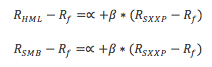
and studied the sign and significance of the intercepts (the ∝).[1]
These regressions both represent, indeed, the CAPM equation, where the risk free rate is subtracted to the dependent variable (the return of the strategy). According to CAPM, the intercepts of these two models should not be different from 0. As for the risk free, we used as a proxy the prices of the one-month futures on the EONIA. In the following paragraph we show the results of the two tests.
We first list some numbers. The average monthly returns of the SXXP index has been 0.63%, while the risk-free rate 0.029%. At the same time, the HML (value) strategy showed a mean return of -0.48%, while the SMB (size) strategy showed a return of 0.72%. If we look at the number of months in which each of the two strategies beat the market, we get a similar feeling. As a matter of fact, the value strategy actually outperformed the SXXP index only 44% of times, less than one-half, while the size strategy beat it 56% of months. The tables below show some key statistics of the regressions that we ran. The first thing to look at is the sign of the intercepts. As we see, for the value strategy the intercept is negative, while it is positive for the size strategy. The interpretation of these coefficients, however, needs first the study of the significance of the two. As we can see, the coefficients are both significant at the 5% level, while only the size strategy presents an intercept which is significant at the 1% level. Even if we are not interested in the beta coefficients, the negative sign of the one of the “size” regression is a puzzling result. In fact, what we were expecting was instead a positive beta for this strategy, given that small companies usually show a systematically higher beta than the one of large companies. The extremely low R^2 of this regression may be an explanation for this.
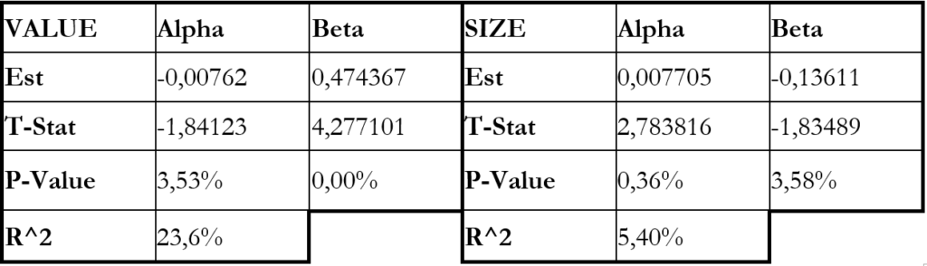
Table 1: Statistics from linear regressions (source of data: Reuters Datastream)
In the chart below we plotted instead the performance, in terms of total returns, of the two strategies, of the SXXP and of the risk free. The starting value is standardized at 100 for all the four investment strategies. As we can see, the Value strategy resulted in losses, while the Size strategy outperformed the market only during last year, when it did not suffer from the bad performance of the market in January.
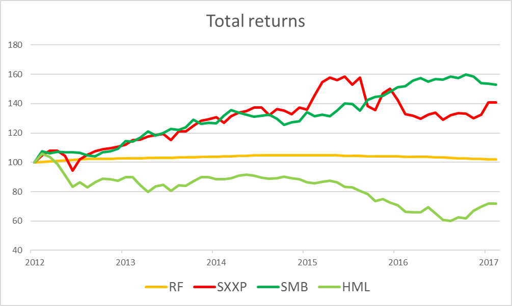
Chart 1: Total returns (source of data: Reuters Datastream)
Conclusions
According to our analysis, the two famous anomalies that were widely discussed and tested during the ‘70s and ‘80s of last century represent no more a “free lunch”. This is consistent with the increased sophistication of modern investors, who analyse in depth every single market in the attempt of exploiting any successful strategy, thus eliminating at least the most easily recognised inefficiencies from the markets.
[1] HML = High-Minus-Low book-to-market stocks. SMB = Small-Minus-Big market cap stocks.


0 Comments