Butterfly trades: Bet on sovereign bonds’ future term structure

Download PDF

Introduction

Following the article from two weeks ago on the barbell and the bullet portfolios, we combine those two strategies together in what is called “butterfly trade”, used by investors to profit mainly on parallel yield curve movements.

This week’s US inflation figures hit hard investors’ confidence. Expectations of even higher inflation jumps in the coming months, have increased pressure on Central Banks policies worldwide. This change in rates environment might affect the volatility and the shape of term structures and butterfly trades can serve as an optimal investments strategy to deal with this level of uncertainty and profit from specific curve movements.

In this article, we present the four main butterfly strategies, discuss how they are structured and explain which exact market conditions must occur to generate positive payoffs when a given butterfly is implemented. Then we will dive deep into the arbitrage opportunities these strategies can help exploiting and finally, based on current market conditions, we detect a butterfly idea by limiting investment risks and maximizing returns.

What is a butterfly?

The butterfly refers to a strategy that aims to exploit the relative value of the “body” versus the “wings” of a three-pronged position. In the fixed income context, the butterfly is a combination of the long barbell (the butterfly’s wings) and the short bullet (the butterfly’s body) or vice versa.

The main idea is to construct a cash (not always) and duration neutral portfolio by adjusting the amount of exposure on long and short bonds. In this investment context, different allocation adjustments allow investors to speculate and profit on predicted fluctuations in the yield curve.

There exist four main types of butterflies: the cash and duration neutral weighting butterfly, the fifty-fifty weighting butterfly, the regression weighting butterfly, and the maturity weighting butterfly.

1. The cash and duration neural weighting butterfly

First, we analyse the traditional cash and duration neutral weighting butterfly. In this strategy, the portfolio is constructed using three different maturities bonds, which are allocated to comply two fundamental conditions: duration neutrality and cash neutrality.

As we mentioned previously, the butterfly is the combination of the short bullet and long barbell, therefore, solving the following system, we determine the weight of each security in the portfolio construction:

Where are respectively the quantity of the short, medium (negative as it is a short position) and long maturities bonds; are respectively the price of the short, medium and long maturities bonds; are respectively the duration of the short, medium and long maturities bonds.

Solving the system of linear equations, we obtain:

To explain the first case, we consider the key property of the butterfly, duration effect is negligible when small parallel shifts occur. Furthermore, we know that the butterfly portfolio usually promises a positive convexity because it offers exposure to the maturities where the price yield relationship exhibits greater curvature than that of its short position. More generally, for a given duration, convexity is higher for more dispersed cash flows, i.e., the barbell exhibits greater convexity than the bullet in the construction of the butterfly because the first contains more dispersed cashflows. To sum up, the parallel shifts of the yield curve generate positive profits as the effect of positive convexity.

Moving to the second case, the decrease in short-term bond prices will be exceeded by the long-term bond’s return gain from price appreciation, as higher maturity securities have higher duration. In a simplified view where the yield of the shorted security is unchanged, to gain from a flattening, the appreciation from the higher maturity security should more than compensate the loss on the short term security. As gains/ losses from the two securities can be approximated by the product of their quantity times modified duration times their change in yield in absolute value, to gain from a flattening the following formula should apply: . This last point is applicable in all the following butterflies’ strategies that we are going to tackle.

The rationale that lies behind coincides with the simple barbell’s mentioned in the previous article and it is applicable in all the following strategies.

1. Fifty-fifty weighting butterfly

Second, we examine in detail the fifty-fifty weighting butterfly. The main idea of this transaction is to structure the portfolio to obtain the same duration on each wing and profit from small steepening and flattening yield movements although the requirements just mentioned in the last case apply.

Some butterfly strategies do not require a zero initial cash flow. In this case, we lose the cash-neutral restriction but maintain the duration neutrality requirement. We determine the weight of each security in the portfolio with the following system of linear equations:

Solving for , we derive:

Thus:

The aforementioned structure generates a positive P/L in both steepening and flattening yield environments. The intrinsic property of this strategy () balances short term securities’ price appreciation (depreciation) with long term securities’ price depreciation (appreciation) in the case both short and long term yield structures experience equal but opposite variations. Moreover, as yield fluctuations become bigger in either direction, the positive effect on P/L becomes larger due to the positive convexity.

Securities’ allocation of the above-mentioned strategy is unbalanced towards shorter-term maturity bonds, because higher maturity securities have higher duration. Moreover, shorter-term securities are priced higher than the longer ones, because of the compounded discounting effect. Therefore, the weighted average of short and long-term bond prices is lower than the price of medium-term maturity. As a consequence, fifty-fifty weighting will require an initial financing cost equal to .

1. Regression weighting butterfly

Third, we explore the regression weighting butterfly. As in the previous two cases, the portfolio is constructed to reflect duration neutrality property. Now, we introduce a new idea, since it is reasonable to assume that some aspects of the past patterns will continue in the future, we believe that there exists a strict correlation between future rates fluctuations with the current and past ones. For example, if historically short term rates have shown to be much more volatile than long term rates, then the same pattern will be reflected in the future.

We determine the weight of each security in the portfolio with the following system of linear equations:

Solving for , we derive:

Note that the fifty-fifty weighting butterfly is a specific case of the regression weighting butterfly with the regression coefficient equal to 1. is the coefficient obtained by regressing changes in the spread between the long wing and short wing using historical data (daily, weekly or monthly changes):

Where are respectively the long term rates variation, short term rates variation and error of the regression at the time i.

This butterfly structure generates a positive P/L both in a flattening curve scenario and when yield curve fluctuations reflect historical patterns (). In such a case, the total duration effect of this portfolio balances short term securities’ price appreciation (depreciation) with long term securities’ price depreciation (appreciation). Moreover, as in the previous scenarios, convexity generates a positive price impact as yield fluctuations become bigger in either direction.

1. Maturity weighting butterfly

Last, we consider the maturity weighting butterfly. This strategy recalls the rationale lied behind the regression butterfly. However, instead of using the historical data to derive the relationship between short and long term rates fluctuations, the idea is to weigh each wing of the butterfly with a coefficient depending on the maturities of the three bonds to satisfy the three following equations:

Where are respectively the maturities of the short, medium and long term bonds, thus:

Solving for , we obtain:

Note that the fifty-fifty weighting butterfly is a special case of the regression weighting butterfly with the regression coefficient equal to . Therefore it generates similar returns in flattening scenarios and depending on its regression coefficient can also achieve curve neutrality.

There is room for risky arbitrages too…

Another way to exploit butterfly trades is to look an arbitrage opportunity. Having defined a butterfly trade as taking long and short positions at different points along the yield curve in a way that zeros out the exposure to the duration of the portfolio, we can apply that to mispricing opportunities. First, an analysis is made to identify points along the yield curve that are either considered “expensive” or “cheap.” Then, the investor enters a portfolio that exploits these misevaluations by going long on the cheap bonds and short on the expensive ones in a way that minimizes the risk of the portfolio and the cash needed to open the trade. Finally, the portfolio is held until the trade converges and the relative values of the bonds come back into line. One thing to remember however is that there could be negative convexity playing against the trader, while the effect is negligible for short maturities, for bonds with high maturity (>10y) and high coupons, the value of convexity plays an important role.

In our case, we assume that the term structure is determined by a two-factor affine model (an affine term structure model is a financial model that relates zero-coupon bond prices to a spot rate model and it is particularly useful for deriving the yield curve) and we fit it to match exactly the one-year and ten-year points along the yield curve each month. Once fitted to these points, we then identify how far off the fitted curve the other yield rates are. Now imagine that for a particular month the market two-year yield rate is more than ten basis points above the fitted two-year yield rate.

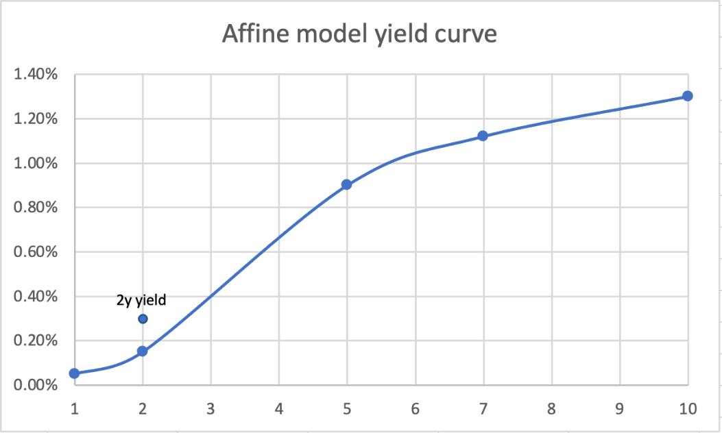
We would enter into a trade by going long of a two-year bond and going short a portfolio of one-year and ten-year bonds with the same sensitivity to the two affine factors as the two-year bond. Once this butterfly trade was put on, it would be held until the market two-year yield rate converged to the model value. The same process continues for each month, with either a trade similar to the above, the reverse trade of the above, or no trade at all being implemented, and similarly for the other maturities.

There also other two more precise methods in determining how the current yield curve is positioned relative to historical relationship and consequently if a bullet is considered expensive with respect to a barbell portfolio or vice versa. Here we will consider the paper written by Tamara Mast Henderson called “Fixed Income Strategy: The Practitioner’s Guide to Riding the Curve” and the two techniques she proposes in evaluating arbitrage opportunities.

In the first technique we plot daily observations in the spread between 5y and 30y against the 2-year yield over a 1-year interval. Then build a scatter plot and compare it to the fitted curve as in the figure below. Points below the fitted curve represent cheapness in the 5-year bonds, while points above the line represent richness. Then once the graph with historical data has been constructed, we point the actual relationship in a specific day (in the example June 11, 2001) and identify it relative to the fitted curve. Based on the relationship presented below, one might expect the 5y/30y spread to widen (i.e. the curve to steepen) – that is, the price of 5-year bonds to rise relative to 30-year bonds. Hence, in this case one would find “value in intermediates”. This translates into entering a long position in 5-year bonds while shorting 2-year and 30-year bonds or in simpler terms that the bullet portfolio is undervalued with respect to a barbell one.

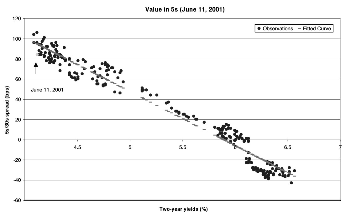
Source: Fixed Income Strategy: The Practitioner’s Guide to Riding the Curve

The second technique involves plotting daily observations of the 2y/5y and 5y/10y spreads against the fitted curve over a 1-year interval. We build again a scatter plot and in this case points above the fitted curve represent cheapness in the 5-year bonds, while points below the fitted line represent richness. Pointing again the actual relationship in a specific day (in the example September 20, 2001) and identify it relative to the fitted curve we find cheapness in the wings this time. Based on the observed historical relationship in this example, one might expect the 5y/10y spread to narrow and the 2s/5s spread to widen – that is, the price of 5-year bonds to fall relative to both 2y and 10y. Hence, a bullet of 5-year bonds would be considered expensive relative a barbell of 2y and 10y.

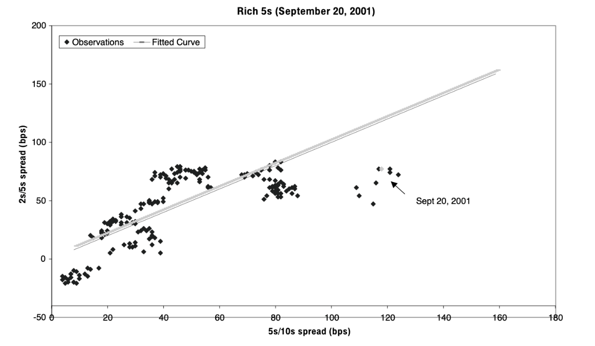
Source: Fixed Income Strategy: The Practitioner’s Guide to Riding the Curve

With the three different techniques described above, butterfly strategies can be considered suitable not just to predict specific movements in the yield curve but also to exploit the misevaluation between barbell and bullet portfolios. One thing to remember however is that for bonds with high maturity (>10y) and high coupons, the value of convexity will also need to be evaluated since it can justify the spreads between the two portfolios’ valuations.

Trade idea

To benefit from the uncertainty on future inflationary pressures and the short term volatility in the Germany yield, we propose to enter a cash neutral butterfly on 5Y-10Y-30Y maturities. Doing so we will benefit from both positive and negative parallel shifts in the long tenor part of Germany’s yield curve.

Germany long term yields rose during last year

Germany yield curve steepened during last year although in the last month is flattening

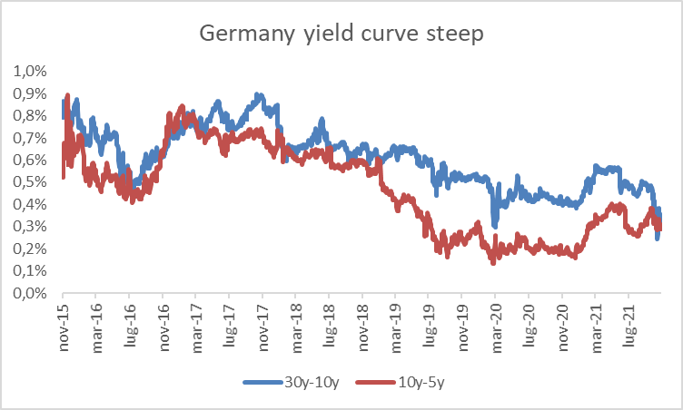
Source: Bloomberg at 14/11/21

We propose to enter a 5Y-10Y-30Y cash neutral butterfly with overall duration equal to zero and positive convexity to benefit from parallel shifts (both upward and downwards) of the German yield curve. We have chosen such maturities as the longer part of the curve is much more dependent from future rates and inflation expectations while front part is more reliant on short term rates policy on which the ECB has reiterated its forward guidance and likely to be steadier. The portfolio is composed as follows:

• A €811M (nominal) long position on the generic 5Y Germany ZCB (DBR 0 10/09/26)
• A €1,000M (nominal) short position on the generic 10Y Germany ZCB (DBR 0 08/10/31)
• A €197M (nominal) long position on the generic 30Y Germany ZCB (DBR 0 08/15/51)

The weights are chosen in such a way to make the duration null, differently the portfolio convexity is positive as the latter is a function of the square of the maturity (while the duration is a linear function). As a consequence the 30y long position positive convexity is dominant.

As shown below the trade has positive outcomes in both upward and downward parallel shifts of the yield curve in the short term, while it is costly to keep it alive.

Moreover a risk of the trade is that the curve steepeners, especially the longer part, increasing the difference between 30Y-10Y yields, posting a loss on the long position of the 30Y bond.

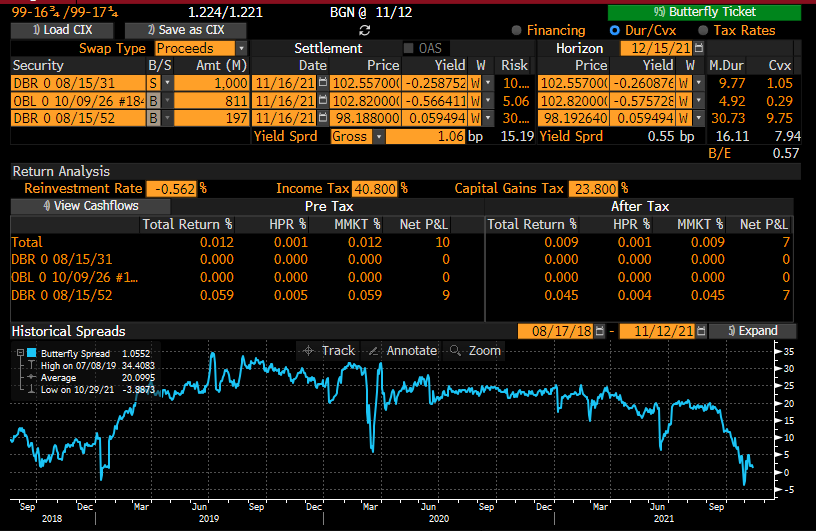
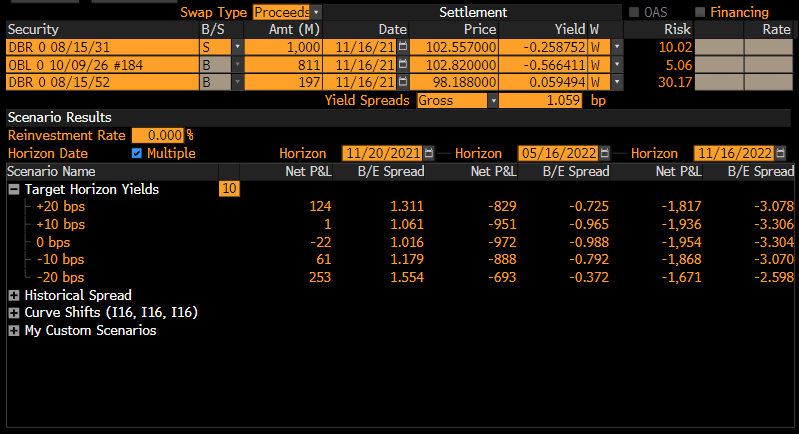
Source: Bloomberg at 14/11/21

References

[1] B. Tuckman, A. Serrat, Fixed income securities, Third edition

[2] L. Martellini, P. Priaulet and S. Priaulet, Understanding the butterfly strategy