EconoMystic Models: The Alchemy of Recession Forecasting

Download PDF

Introduction

Headlines over the last few months have been constantly showing investors and economists discussing the various “landing” narratives for the US economy. With many arguing for a soft-landing scenario, while others remained more skeptical. At its core, this debate revolves around a critical question: “What are the odds of a recession?”

Predicting recessions and estimating their likelihood has been a continual challenge for market practitioners, policymakers, and academics. In this article, we present the implementation of the profit regression model in the field of recession forecasting, along with our own estimates of US recession probabilities for 3, 6, 9 and 12 months ahead. Through this analysis, we seek to disentangle the alternative narratives by dissecting the results of the models and assessing their relevance in the current macroeconomic landscape.

Recession Basics

What is a recession? The answer to this question seems to be straightforward, but in reality, it is much more complicated than it appears. The issue is that no official definition of recession exists, although there is general recognition that the term refers to a period of decline in economic activity.

Most commentators and analysts define it in practice as “Two consecutive quarters of decline in a country’s real gross domestic product”. This definition may be a useful rule of thumb, nevertheless focusing on real GDP alone is not enough. On the other hand, national statistical agencies, central banks, and other international institutions have their own criteria for determining and declaring recessions.

In the case of the US economy, the NBER’s Business Cycle Dating Committee defines a recession as “A significant decline in economic activity spread across the economy, lasting more than a few months, normally visible in real GDP, real income, employment, industrial production, and wholesale-retail sales. […]”.

Instead, for the Eurozone, the Euro Area Business Cycle Network (EABCN) defines recessions as “A significant decline in the level of economic activity, spread across the economy of the Euro Area, usually visible in two or more consecutive quarters of negative growth in GDP, employment and other measures of aggregate economic activity for the Euro Area as a whole”. While the EABCN definition applies for recessions for the entire Eurozone, the single member economies still use their own chronologies and definition.

Another layer of complexity is added when we compound the fact that the process of determining whether a country has fallen into a recession or not often takes time. This is understandable. The decision process considers many variables, which are often subject to seasonal revisions after their initial announcement. Thus, it is very likely that by the time a recession is officially announced, the economy is already in a state of decline.

Recession Forecasting

Many economic players are interested in predicting recessions and changes in future economic activity for different reasons, ranging from risk mitigation, portfolio reallocation, and the implementation of counter-cyclical economic policies.

A variety of models have been developed for this specific purpose, ranging from simple OLS regression to Vector Autoregressions (VARs), but also including some machine learning models such as Support Vector Machines (SVMs). Among these models and the extensive academic literature on the subject, in this article we will present and analyze the probit model, one of the most popular non-linear models in the field of recession forecasting as presented by Estrella (1998).

Probit Model

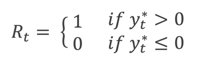
Probit regression, also called a probit model, is a binary response model. The model assumes an unobservable latent variable for which there exists a binary outcome variable denoting the occurrence or non-occurrence of an event. In our case we consider:

• The latent variable , which represents the state of the economy
• The outcome variable which takes value of 1 when the economy is in recession, and 0 otherwise:

The latent variable linearly depends on

*** QuickLaTeX cannot compile formula:
 

*** Error message:
Error: Nothing to show, formula is empty

, which is the set of explanatory variables, including a constant, according to:

where is the length of the forecast horizon, is a vector of parameters, and is a normally distributed and homoskedastic error term:

The probability that the economy is in a recession at time , i.e., is:

The vector is estimated using MLE, that is by maximizing the likelihood function:

The Data

We considered for our analysis monthly datapoints, which span from 01/01/1960–30/09/2023. Our probit model utilizes official NBER recession dates as recession indicator . We attempt to compute recession probabilities using different individual known leading indicators encompassing:

• The difference between 10-year and 3-month treasury yields (10y–3m). We use this spread instead of more widely cited spreads by practitioners such as the 10y–2y or the 10y–1y, due to better predictive power of the former (Bauer and Mertens 2018b). The spread is computed using monthly averages instead of end-of-month rates, as there is evidence that end-of-month data may contain systematic biases (Park and Reinganum 1986).
• The Conference Board US Leading Economic Index (LEI), which is designed to signal peaks and troughs in the business cycle. The LEI has ten components, including metrics such as average weekly initial claims for unemployment insurance, the S&P500 index, and the 10y minus fed funds spread (for more details please check here). For our analysis we will use the yoy% change of LEI.

Evaluation Criteria

We will evaluate the model fit using three criteria:

1. as proposed by Estrella (1998), defined as

where denotes the estimated likelihood of the current model considering all explanatory variables, is the estimated likelihood of the null model (i.e., with only constant). This metric measures the goodness of fit of the model.

1. Area Under the Receiver Operating Characteristic Curve (AUC–ROC), computed as

where r is defined as the false positive rate (FPR).

The ROC curve is the graphical representation of the effectiveness of the binary classification model. It plots the true positive rate (TPR) vs the false positive rate (FPR) at different classification thresholds. The performance metric AUC-ROC quantifies the overall ability of the model to discriminate between the positive and negative classes, irrespective of the threshold.

1. Balanced Accuracy (BA) which is defined as the average of recall obtained on each class, which means it accounts for both the true positive rate and the true negative rate, computed as

where TP is the number of true positives, TN the number of true negatives, FN the false negatives, and FP the false positives.

This metric is used to evaluate classification models, especially when dealing with imbalanced datasets, such as in our case, by giving a fairer evaluation of the classifier’s performance.

In-sample evaluation

We first run the probit regression using the whole dataset (01/01/1960–30/09/2023) and then we compare the actual recession dates with the fitted values at forecasting horizons of 3, 6, 9, 12, 15, and 18 months ahead. For the sake of our analysis, we decided to choose a classification threshold of 0.20 which we deemed to be the most appropriate level.

We find that over the short forecast horizons of 3 and 6 months ahead, the models with the Leading Economic Index (LEI) as explanatory variable outperform the 10y–3m spread in terms of both model fit and accuracy.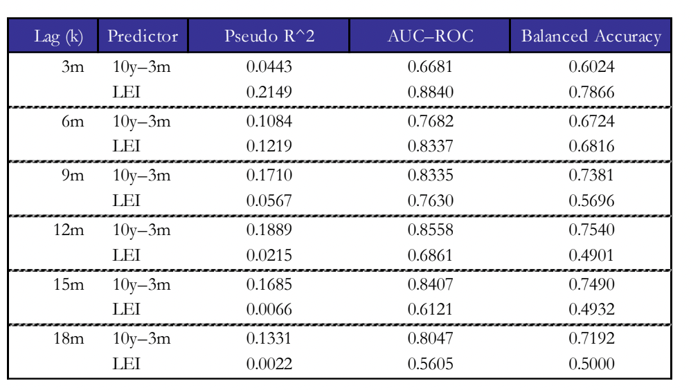Source: Bocconi Students Investment Club

Nevertheless, already starting from 9 months ahead, the goodness-of-fit and accuracy measures for LEI start to rapidly deteriorate, whereas the same metrics for the 10y–3m spread improve, showing good predictive power over different time horizons.

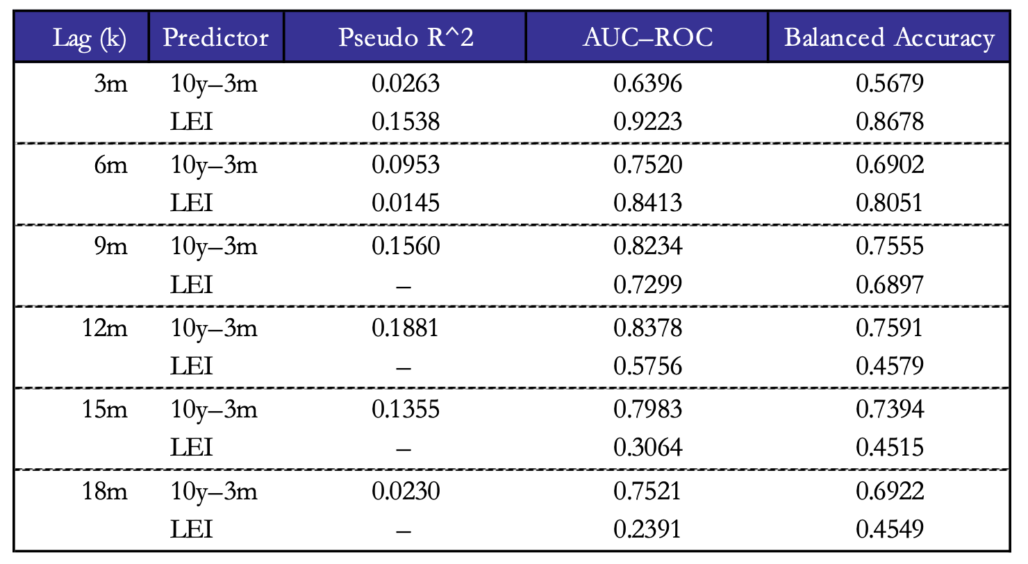
Expanding window evaluation

In the previous section the models may give rise to overfitting as they are tested on the same dataset on which they are trained. Overfitting gives a false sense of model effectiveness, as the model may show high accuracy during testing but will perform poorly on unseen data.

In order to assess in a fairer and more realistic way the forecasting power of the model we use an expanding window. In simple words, the results are obtained by first estimating the model with a predefined initial set of data, which we set to 120 observations (i.e., 10 years of data) to avoid perfect separation. The model is then used to make predictions months ahead. Subsequently we include an additional month of data in in the training set, and the entire procedure is repeated.

A downside of the expanding window forecasting is that the metric may not always lie between 0 and 1. This is due to the differences between in-sample and out-of-sample data which can lead to inconsistencies in the interpretation of the . Therefore, we decided not to consider negatives values of the metric in this section, which are just signs of poor forecasting performance.

Source: Bocconi Students Investment Club

The out-of-sample results reconfirm what we already stressed for the in-sample models. The LEI shows better forecasting accuracy at shorter horizons (3m, 6m) compared to the 10y–3m spread, which however displays more consistent predictive power across all the lags considered.

Real-time US Recession Probabilities

What are the current recession probabilities for the US economy? How have these probabilities changed during the past year?

In order to answer these questions, we trained the probit models presented in the previous sections using data available until 2021. The models were then utilized to compute the recession probabilities for the horizons of 3, 6, 9, and 12 months ahead starting from January 2022 until September 2023.

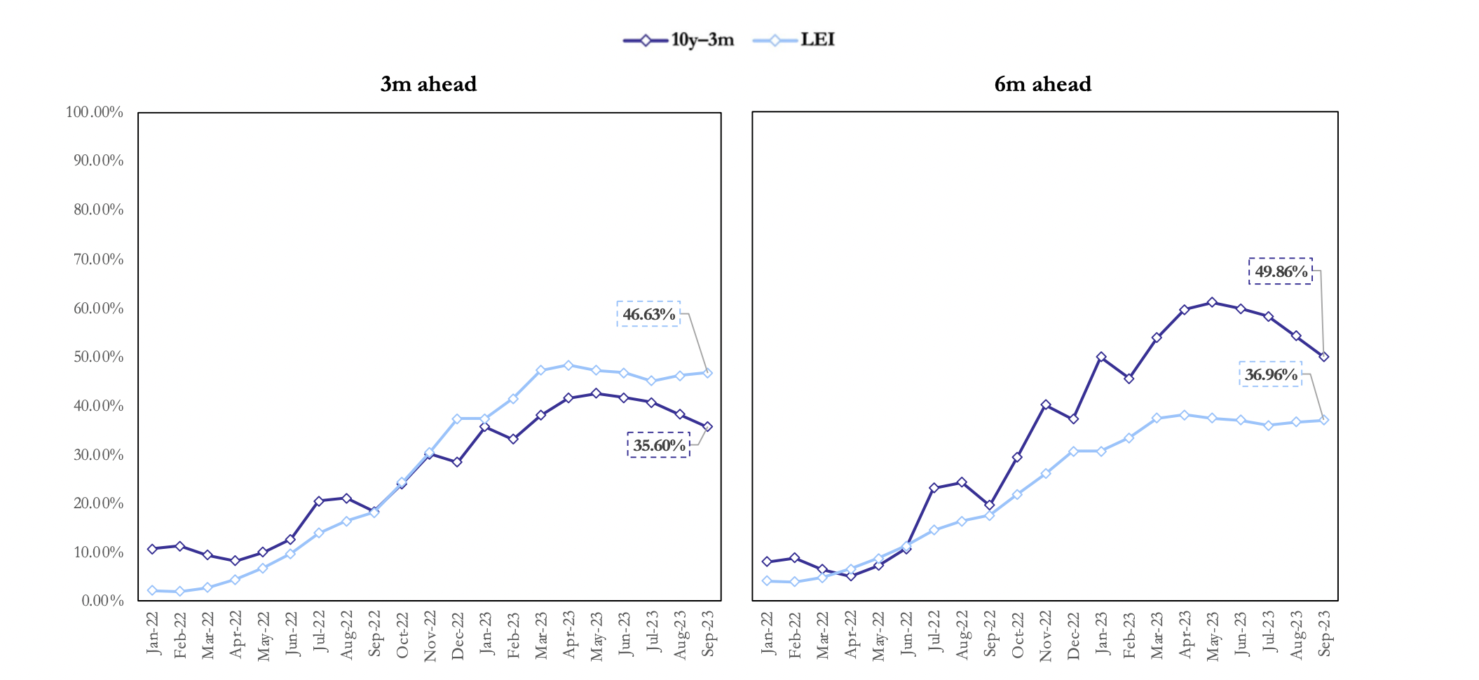
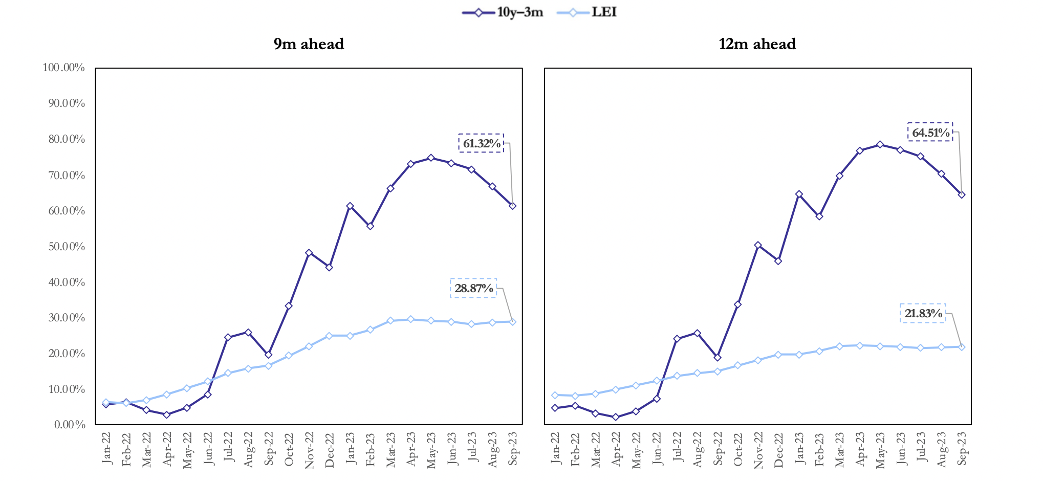
Source: Bocconi Students Investment Club

As shown by the charts above, the recession probabilities computed by the models have been increasing both for the LEI and the yield curve data over all time horizons since early 2022. In particular, the probabilities obtained from the 10y-3m term spread data show values of 61.32% and 64.51% respectively for 9 and 12 months ahead, the horizons in which the fit of the yield curve indicator outperforms the LEI. The latter assigns, in fact, higher probabilities for shorter time horizons, with the highest probability assigned at the horizon of 3 months ahead, at 46.63%.

Okay, but now what?

Throughout the Fed’s hiking cycle, the US economy has shown high levels of resilience, with the impressive reading of GDP growth for Q3 surprising markets to the upside coming out at a 4.90% yoy, the highest since Q4 2021 while the unemployment rate is still at historically low levels at 3.90% in October. By looking at these numbers one could assume that we are indeed in a “goldilocks” scenario in which the US economy is calmly shrugging off 500bps of rate hikes. Nonetheless, these numbers do not tell the whole story.

The unemployment rate, albeit historically low, is close to triggering the “Sahm rule” (Sahm 2019), according to which a recession occurs when the three-month moving average (currently 3.83%) of the unemployment rate (U3) rises 50bps above its minimum over the previous 12 months (currently 3.50%). Furthermore, Friday’s NFP data came in lower than expected at 150,000 versus expectations of 180,000, while September’s numbers were revised down to 297,000. The ISM manufacturing PMI came in at 46.7, surprising markets to the downside. All signs of a slowing economy in the US, which the market took well, with stocks, bonds, and gold gaining while the USD fell amid falling yields.

The Fed, as well as Treasury’s Janet Yellen have, in fact, welcomed the recent bear steepening as higher rates on the long end of the yield curve are those that impact real economic activity putting pressure on corporates and households intending to issue debt and bond markets seem to be “doing the Fed’s work” in tightening financial conditions. According to LSEG data, the month of October has been the slowest since 2011 in terms of issuance, with US corporates issuing just over $70bn in the month across just 50 deals, the lowest number in 20 years.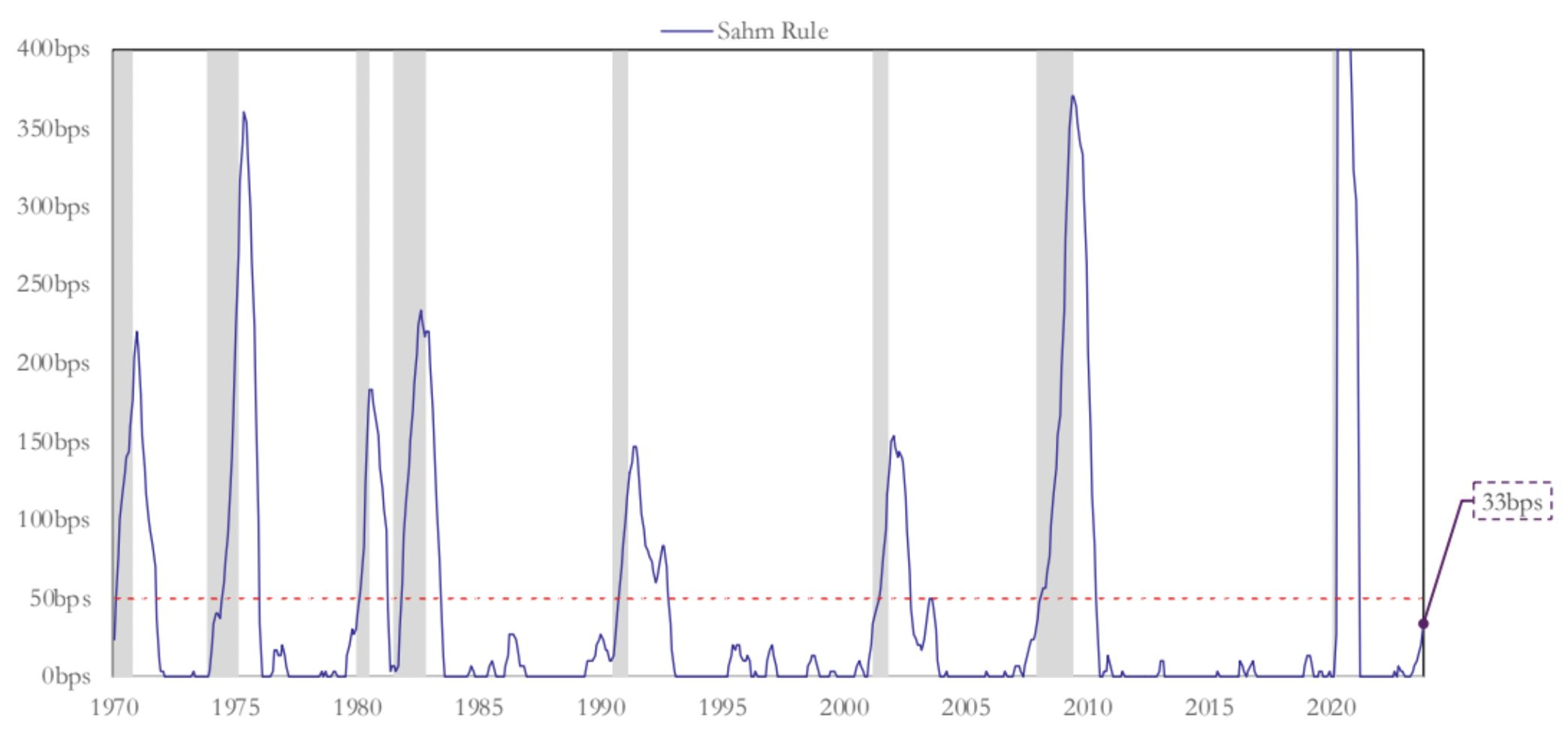Source: Bocconi Students Investment Club, FRED

Regarding the steepening of the yield curve, it is important to note the decline in the probabilities computed with the yield curve indicator in the last few months. This is because, as the curve steepens, the inversion declines and so does the signal upon which probabilities are computed. Recessions have historically been preceded by this pattern, albeit a bull steepening rather than a bear steepening since investors begin pricing in cuts in the short end before recessions as the central bank is expected to ease its monetary stance to support the economy. The Fed, in this case may welcome an economic slowdown to bring inflation back to target.

Behind the strong GDP numbers was the resilience of US consumers, with consumption growth representing around half of the 4.90% growth. However, consumers tell another double-faced story: while they continue to spend, they keep a pessimistic view of the future with the Conference Board’s consumer confidence index down for the third consecutive month in October, reaching 102.60. Notably, the “Present Situation Index” declined to 143.10 and the “Expectations Index” fell slightly to 75.60. An Expectations Index below 80.00 has historically indicated an incoming recession in the next 12 months, especially when there is high divergence with the Present Situation Index.

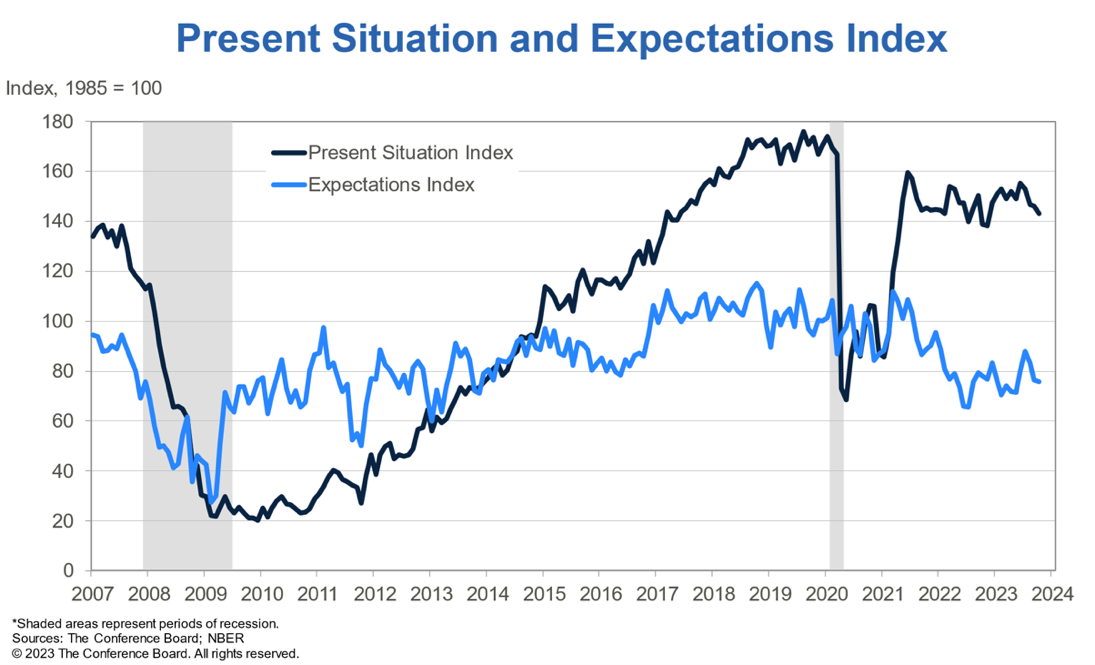
Source: The Conference Board, NBER

The divergence of narratives in the US economy is reflected in market prices of different asset classes, long term treasuries (iShares 20+ Year Treasury Bond ETF TLT) are down more than 40.00% from the 2021 highs while the S&P500 is down just about 10.00% from the 2021 highs. In the current environment, stock prices should head lower: on the one hand the mere level of interest rates and the rising term premium should be reflected in a decreased present value of future cash flows and on the other hand, earnings growth should be revised down due to more stringent monetary conditions that will slow the growth fueled by cheap debt in the past years, as well as overall demand. The only reason for high equity valuations would be with high double-digit earnings growth, which however is inconsistent with high recession probability.

Another asset class currently priced for a soft-landing scenario seems to be credit, especially HY credit space: the current option-adjusted spread (ICE BofA US High Yield Index Option-Adjusted Spread) is at 4.15% versus an historical average during times of recession of 9.36% and a long-term average of 5.38%, indicating that HY credit is not incorporating the risks associated with the current environment.

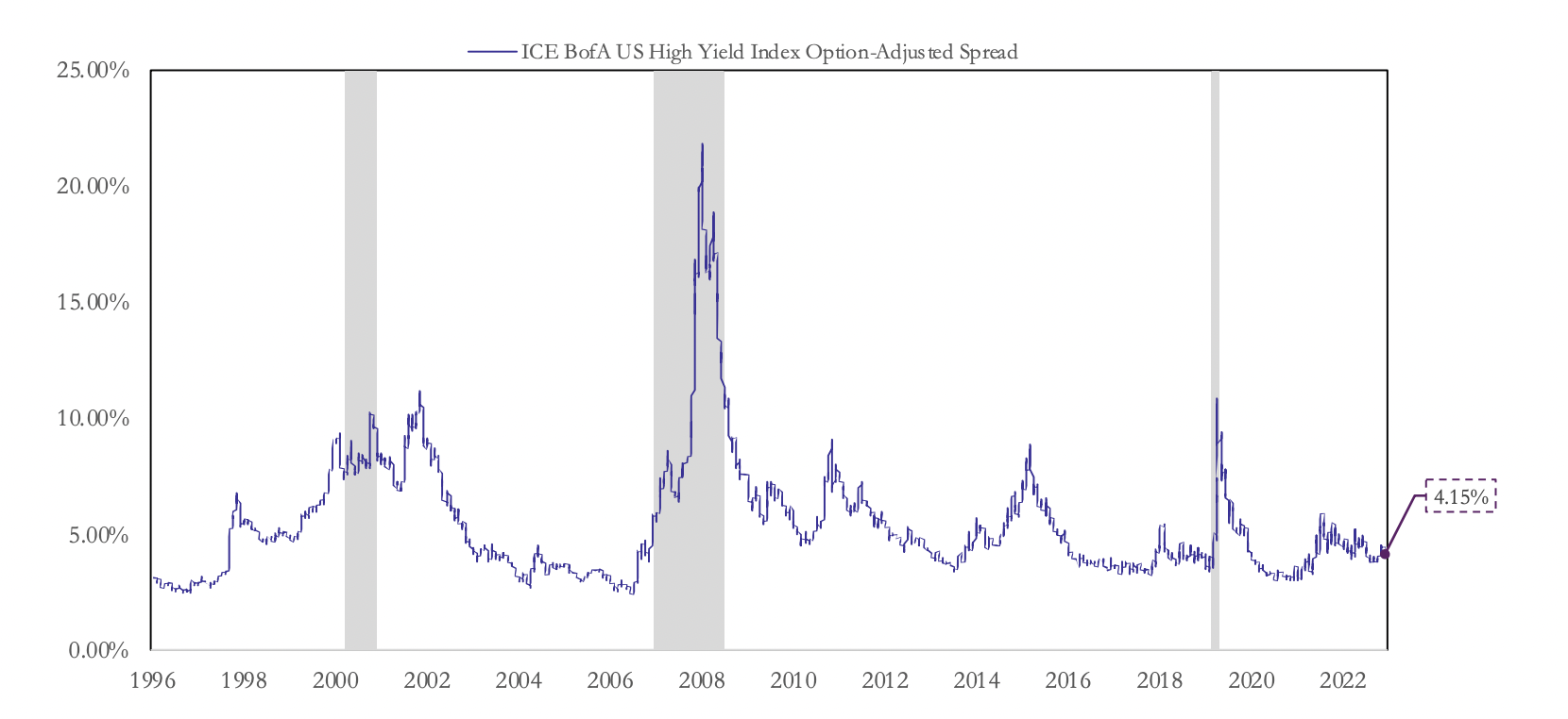
Source: Bocconi Students Investment Club, FRED

Overall, both the results obtained from the probit models and market pricing indicate a high degree of uncertainty around the US economy, as there is currently no consensus view around the present situation in neither expert opinions nor in the data. However, it is important to note that clear signs of the US economy slowing down are appearing and the market may not be pricing all the risks associated with a non-negligible recession probability in the upcoming months.

Conclusions

This article presented one of the many models used to try to predict recessions and aimed at informing the reader about the relevance of the results obtained through this analysis in a period of high uncertainty in which the US economy seems to remain strong despite severe monetary tightening by the Fed and where “good news is bad news”.

Finally, as the title of the article suggests, there is no “best” way to predict recessions as many approaches have been tried and no model clearly prevails on all the others. Furthermore, to quote Bohr (or Nostradamus, or Yogi Berra, or no one?) “It is difficult to make predictions, especially about the future”, and we would like to add “especially if we do not actually know what we are trying to predict”, since there is no consensus definition of recession. We believe that continued research in this field is needed, as better information on the economic cycle may lead to improvements both from a policymaking and an investment perspective, thus increasing overall welfare.

References

[1] Bauer A. and Mertens T., “Information in the Yield Curve about Future Recessions”, 2018b, FRBSF Economic Letter.

[2] Estrella A. and Mishkin F., “Predicting U.S. Recessions: Financial Variables as Leading Indicators”, 1998, The Review of Economics and Statistics, 80(1):45–61.

[3] Horowitz J. and Savin N., “Binary response models: Logits, probits and semiparametrics”, 2001, The Journal of Economic Perspectives, 15(4):43–56.

[4] Park S. Y. and Reinganum M., “The puzzling price behavior of treasury bills that mature at the turn of calendar months”, 1986, Journal of Financial Economics, 16(2):267–283.

[5] Sahm C., “Direct stimulus payments to individuals”, 2019, Recession ready: Fiscal policies to stabilize the American economy, pages 67–92.