Half a Century of Black-Scholes: Option Pricing Models from Inception to Contemporary Innovations

Download PDF

Introduction

50 years ago, the financial industry changed forever with the introduction of the Black-Scholes model for options pricing. However, the story started much earlier with less sophisticated approaches and has evolved significantly over the last century, encompassing notable frameworks such as the binomial tree in discrete time, and more sophisticated models accounting for stochastic volatility. This article takes you through the journey of option pricing models from the early foundations to the most recent innovations, examining the pioneering role of the Black-Scholes model and its enduring impact 50 years later.

The Beginnings of Option Pricing

As reported by Sullivan and Weithers (1991), options were historically viewed as esoteric financial instruments. They appeared in the fourteenth century as insurance contracts related to shipments in the Mediterranean. In the seventeenth century, however, option contracts became popular as hedging and speculative devices in the Dutch tulip market. By the end of the century options had developed a bad reputation due to excessive speculation and the lack of margin requirements. These contracts however, periodically re-emerged in many European exchanges. Among these, La Bourse (the Paris exchange) had developed, by 1900, a well-organized market for equities, bonds, futures, and options.

In this framework the man who is considered the “father” of option pricing introduced a first model to systematically price option contracts. On March 19, 1900, Louis Bachelier defended his doctoral thesis Théorie de la Spéculation, in which he anticipated many of the foundations in modern option pricing models and financial markets in general. When it comes to options, the first innovation brought about by Bachelier is the standard option payoff diagram at maturity that shows a flat line until the strike price and then grows linearly in the underlying price. His studies focused only on the study of options that could be exercised at maturity i.e., European.

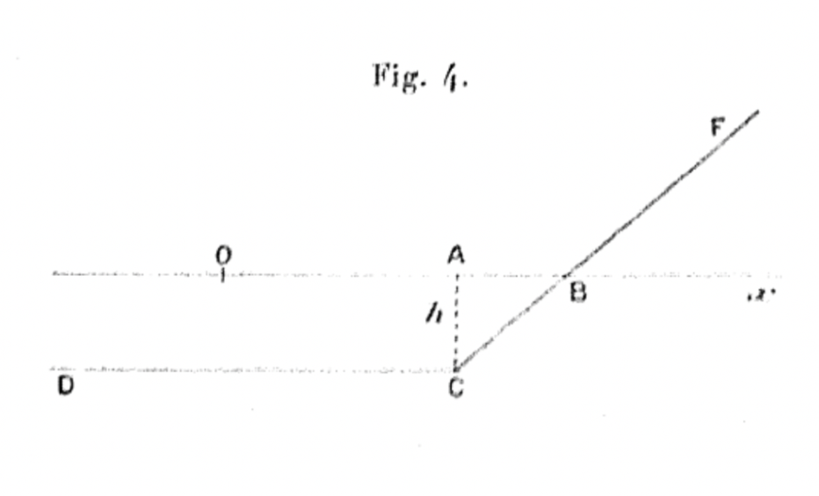Source: Louis Bachelier, “Théorie de la Spéculation”, 1900.

Furthermore, to understand the pricing of options, Bachelier’s study had to focus on the behavior of the underlying stocks. He assumed changes in the stock price to be identically and independently distributed, forming the basis for the efficient market hypothesis, according to which current prices reflect all available information, thus making future returns independent of past returns as they reflect different information. A famous quote from his thesis states that “the mathematical expectation of a speculator is null”. In this way, he introduced the concept of Brownian motion to financial markets, as, according to his model stock prices followed such a stochastic process, albeit an arithmetic one that has since been replaced by a geometric Brownian motion since the former assigned positive probabilities to negative stock prices, inconsistent with limited liability securities such as equities.

The formula to calculate the premium of a call option according to Bachelier’s model can be written as:

Where this price is just the expected difference between (the stock price at T) and K (the strike price) weighted by p, the probability that the price at T is .

1960s – Evolutions Leading to Black-Scholes

Until the 1960s, Bachelier’s work on option pricing was known to a small niche of mathematicians and his contribution to financial economics was not appreciated. In the fifties, however Paul Samuelson “was able to locate by chance this unknown book, rotting in the library of the University of Paris”, this book was indeed Bachelier’s thesis. Following this discovery, Samuelson commissioned the translation of this book to James Boness, contained in Cootner (1964). In that period Samuelson and Boness were working on finding discounted payoffs for European options. Boness, in his PhD dissertation (1962) obtained a formula that laid the groundwork for the later Black-Scholes option pricing formula, as well as discussing how it is never optimal to exercise American call options early and how it can be optimal for puts.

Boness’ formula can be interpreted as follows: let A be the expected value of the truncated probability distribution of only favorable future prices (i.e., when the option is in-the-money) and B the probability of having favorable prices, then the value of a call at maturity will be, similarly to what obtained by Bachelier, (A-K)B, the present value of the call will be discounted at the expected rate of return of the underlying security and, translated in a more recognizable fashion, the price of a European call option on asset i will be:

Where: is the value of the option at time t, K is the strike price of the option, is the stock price at time t, T is the maturity date, N is the cumulative normal distribution, is the stock’s volatility.

The assumptions underpinning this model are quite different from those of the Black-Scholes model, nonetheless the pricing formulae are strikingly similar, with the only difference being the presence of the expected return of asset i instead of the risk-free rate both as a discounting factor and inside and . As reported by Galai (1978), Boness’ model only assumed that markets are in equilibrium, percentage changes in stock prices are lognormally distributed and stationary, and investors are risk neutral.

In 1967 Kassouf and Thorp published an empirical formula for option pricing and introduced the concepts of hedge ratio and dynamic hedging, which will become pivotal in Black-Scholes. The empirical work of Thorp, combined with Boness’ formula led him to the final intuition that brought him to the Black-Scholes formula. In fact, he substituted the expected return of the underlying security with the risk-free rate, effectively reaching the Black-Scholes formula, which he successfully used for trading without being able to prove why it worked.

1973 – Arrive Black, Scholes… and Merton

In 1973’s seminal paper “The Pricing of Options and Corporate Liabilities” Fisher Black and Myron Scholes were finally able to mathematically reach the notorious options pricing formula used to this day across the world. Building on the previous literature explored in this article, they were able to prove the formula in two different ways: the first argument is based on no arbitrage and the second is based on the CAPM. The assumptions underlying the Black-Scholes model are the following:

1. The short-term interest rate is known and constant through time,
2. Stock prices follow a geometric Brownian motion in continuous time with variance proportional to the square of the stock price, the variance rate is constant. Thus, stock prices after a finite period are log normally distributed,
3. There are no transaction costs,
4. Assets are infinitely divisible i.e., agents can borrow any fraction of the stock at the risk-free rate,
5. There are no limits on short selling.

Under these assumptions the price of an option is just a function of the price of the underlying stock and of time c(S, t). The first no-arbitrage argument relies on the construction of a hedging portfolio consisting of a long position in the stock and a short position in where the denominator is just the partial derivative of the option value with respect to the stock price. It is easy to understand how such a portfolio (if dynamically hedged as understood by Kassouf and Thorp (1967)) bears no risk. For every unit change in the underlying stock, the option value will change by a value equal to its the partial derivative with respect to the stock price and by having this at the denominator the change will be normalized to one, thus completely balancing out the unit change in the stock price. Indeed, continuous hedging is needed as, with changes in S and t, the number of options to short sell changes. Since, thanks to dynamic hedging, this portfolio is effectively riskless, its return must be the risk-free rate. Using stochastic calculus from this portfolio, they obtained the notorious partial differential equation (PDE) reported below, whose boundary conditions (the payoff diagram at maturity) provide the option pricing formula.

The final option pricing formula will be the same as the one found by Boness, with the only exception that the return of stock i is replaced by the risk-free rate. Interestingly, as stated by Galai (1978), Boness reached his pricing formula by discounting the expected payoff for the option, while Black and Scholes found the pricing formula by solving the PDE describing the behavior of the hedging portfolio.

The second argument, based on the CAPM, relies upon the fact that the analyzed portfolio will have beta = 0 and its return will therefore be the risk-free rate, thus reaching the same PDE. Before the Black-Scholes paper was published, Merton (1973) provided an alternative derivation to the Black-Scholes formula, recognizing that the portfolio will not just be zero-beta but rather its returns are non-stochastic. This led to a more robust derivation of the PDE whose boundary condition leads to the option pricing formula.

A Simple Empirical Example

We now go through an empirical evaluation of the Black-Scholes option pricing using data for AAPL as of September 22, 2023. The risk-free rate is assumed to be the 90-day T-Bill rate and the stock is assumed to follow a geometric Brownian motion of the form

where

is the stock’s expected return and W is itself a standard Brownian motion that produces the stochastic nature of the paths and we subtract the present value of dividends.

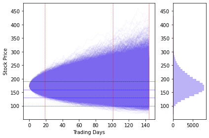
Source: Yahoo Finance, Bocconi Students Investment Club

The previous graph reports 100,000 simulated paths for the price of AAPL, the vertical lines represent the analyzed expiration dates and the horizontal lines the analyzed strike prices. The resulting distribution of terminal stock prices presents a clear rightward skew (in the image upward due to the orientation) as expected since it should represent a log normal distribution. The following table reports the calculated prices for AAPL options using the BS formula and by discounting the average payoffs of options in the simulated paths.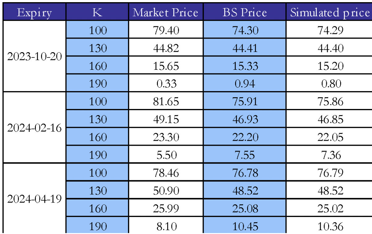

Source: Yahoo Finance, Bocconi Students Investment Club

The calculated prices follow very closely the market price for the traded options and, unsurprisingly, the simulated prices and the Black-Scholes prices result almost identical as they are based on the same assumptions, both presenting a root mean squared error (RMSE) of ~ 2.65.

Option Pricing After Black-Scholes

By working with the Black-Scholes model and a stock price model featuring Poisson jumps, Cox and Ross (1974) introduced the concept of risk neutrality, they hypothesized (but were unable to formally prove) that in some generality the price of an option can be computed with preferences such that expected returns for both the stock and the option are equal to returns under the risk-free rate. By making the same assumptions as BS and by denoting the price of the option by the continuous function P(S, t) the jump process will be of the form:

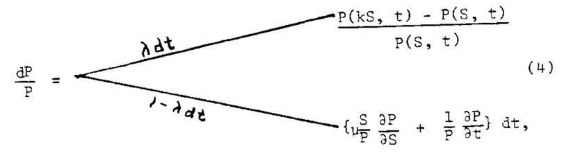
Source: Cox and Ross, “The Pricing of Options for Jump Processes”, 1974.

In other words, the option price will jump to P(kS, t) with probability and otherwise, it will just change due to the exponential nature of the underlying with the passage of time.

A formalization of the Cox-Ross results came in Harrison and Kreps (1979), where the authors proved that the “preferences” found in Cox-Ross must be such that the discounted price processes are martingales (i.e., stochastic processes whose expected value for the next observation is the last observation:). This led to the introduction of equivalent martingale measures, upon which much of subsequent developments in financial markets are based. In the same year Cox, Ross, and Rubinstein (1979) published a paper containing the notorious binomial tree model for option pricing in discrete time, where at each step the stock price can move up or down by a given factor and with a given probability, showing how stock prices conform to a limiting form of discrete binomial process. This paper gives a very intuitive way of pricing options and, as stated by the authors “the simple two-state process is really the essential ingredient of option pricing by arbitrage methods. This is surprising, perhaps, given the mathematical complexities of some of the current models in this field. But it is reassuring to find such simple economic arguments at the heart of this powerful theory.”

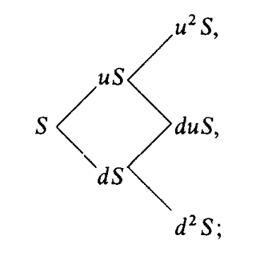
Source: Cox, Ross and Rubinstein, “Option Pricing: A Simplified Approach”, 1979.

Further developments came in the 1990s, when many academics developed models that addressed one of the key problems in the Black-Scholes model, namely the constant nature of volatility, as the model was unable to explain the volatility smiles and skews present in markets. The first model to reach a closed-form solution for option prices under stochastic volatility is presented in Heston (1993), where the variance of the Brownian motion followed by the underlying price is itself a mean-reverting stochastic process, where the instantaneous variance reverts to the long-run variance at a speed to be calibrated according to the data. Further work by Heston can be found in Heston and Nandi (2000), where the authors developed a closed-form solution for option pricing in a discrete-time GARCH framework. Another seminal paper analysing the non-constant nature of volatility is Dupire (1994), who introduced the concept of local volatility i.e., where volatility is expressed as a function of the underlying price and time. From the approaches trying to overcome Black-Scholes, Dumas, Fleming and Whaley (1998) re-evaluate the BS model. Their results can be summed up in 3 words found in the paper’s conclusion: “simpler is better”. This paper was the beginning of the “Practitioner Black-Scholes” where volatility is estimated by a cross-section of implied volatility across strikes and prices.

Lassance and Vrins (2017) advocate, much like Dumas, Fleming and Whaley, in favour of simpler approaches, in their paper they show that more complicated models like Heston-Nandi or Heston, while improving pricing accuracy, do not bring any improvements when it comes to hedging due to the time instability of the parameters.

In conclusion, as the world of finance continues to evolve, powered by advancements in computational capabilities and increasingly complicated assets traded, option pricing is increasingly veering towards numerical methods. From Monte Carlo simulations (as explained by this BSIC article) to Finite Difference methods in jump diffusion and Lévy processes as presented by Andersen and Andreasen (2000) and Cont and Voltchkova (2004). While this article provided a snapshot of the historical models that have shaped option pricing – from the Black-Scholes to Heston models – it merely scratches the surface of the innovative techniques being deployed in modern-day trading floors.

References:

[1] Andersen, L., and Andreasen, J., “Jump-Diffusion Processes: Volatility Smile Fitting and Numerical Methods for Option Pricing”, 2000, Review of Derivatives Research

[2] Bachelier, L., “Théorie de la Spéculation”, 1900

[3] Black, F., Scholes M., “The Pricing of Options and Corporate Liabilities”, 1973, Journal of Political Economy

[4] Boness, J.A., “Theory and Measurement of Stock Option Value”, 1962

[5] Cont, R., Voltchkova, E. “A Finite Difference Scheme for Option Pricing in Jump Diffusion and Exponential Lévy Models”, 2003

[6] Cootner, P.H., “The Random Nature of Stock Market Prices”, 1964

[7] Cox, J.C., Ross, S.A., “The Pricing of Options for Jump Processes”, 1974

[8] Cox, J.C., Ross, S.A., Rubinstein, M., “Option Pricing: A Simplified Approach”, 1979, Journal of Financial Economics

[9] Dumas, B., Fleming, J., Whaley, R.E., “Implied Volatility Functions: Empirical Tests”, 1998, Journal of Finance

[10] Dupire, B., “Pricing with a Smile”, 1994, Risk

[11] Galai, D., “On the Boness and Black-Scholes Models for Valuation of Call Options”, 1978, Journal of Financial and Quantitative Analysis

[12] Harrison, J.M., Kreps, D.M., “Martingales and Arbitrage in Multiperiod Securities Markets”, 1979, Journal of Economic Theory

[13] Heston, S.L., “A Closed-Form Solution for Options with Stochastic Volatility with Applications to Bond and Currency Options, 1993, Review of Financial Studies

[14] Heston, S.L., Nandi, S., “A Closed-Form GARCH Option Valuation Model”, 2000, Review of Financial Studies

[15] Kassouf, S.T., Thorp, E.O., “Beat the Market: A Scientific Stock Market System”, 1967

[16] Lassance, N., Vrins, F., “A Comparison of Pricing and Hedging Performances of Equity Derivatives Models”, 2017

[17] Merton R.C., “Theory of Rational Option Pricing”, 1973, The Bell Journal of Economics and Management Science

[18] Sullivan, E.J., Weithers, T.M., “Louis Bachelier: The Father of Modern Option Pricing Theory”, 1991, The Journal of Economic Education