Introduction
The purpose of this article is to apply the mathematical framework of Modern Portfolio Theory to an unconventional asset class. Cryptocurrencies, Bitcoin included, are a novel and little known asset class with a relatively low market cap of $44 billion and very high volatility.
By applying Markowitz’s Portfolio Theory we intend to take advantage of the joint variability of assets (i.e. covariance) to reduce the overall volatility of the portfolio. Indeed our findings, consistently with MPT, are that portfolio variance can be significantly lowered by exploiting low covariances between coins.
Firstly, we are going to present a general overview of Modern Portfolio Theory, then a short note on methodology, a brief description of each cryptocurrency taken under scrutiny and finally the implementation of the portfolios.
Modern Portfolio Theory
Economist Harry Markowitz in his famous paper “Portfolio Selection” (1952) pioneered the theory of portfolio selection, for which he was later awarded the Nobel Prize. The key assumptions of MPT are that investors are expected return maximizers and risk-averse, meaning that they face a trade-off between portfolio variance and expected return.
In the model, portfolio expected return is defined as a combination of individual assets’ return:

Where:

Note that each weight must be greater or equal to zero (i.e. no short sales) and the weights must sum to one.
Portfolio variance is a function of covariances of the assets pairs:

Where:

For a detailed explanation of the mathematical derivation of the previous formulas we invite the reader to consult the original 1952 paper by Markowitz, easily available online.
A key insight of MPT is that investors can reduce portfolio variance through diversification, by holding assets that are not perfectly positively correlated. Indeed, if assets pairs are perfectly positively correlated (ρ=1), portfolio variance is the sum of each asset’s variance weighted by its proportion in the portfolio (maximum variance) while in case pairs are perfectly uncorrelated (ρ=0), portfolio variance is the sum of each asset’s variance weighted by the square of its proportion in the portfolio.
By graphing different portfolios in a mean-variance diagram, it is possible to observe a characteristic parabolic shape, the ‘Markowitz bullet’, where the upper boundary is called the ‘efficient frontier’: the set of portfolios with the minimum variance for a given expected return or, alternatively, the set of portfolios with the highest expected return for a given variance. The bottom-left portfolio of the efficient frontier is called the ‘global minimum-variance’ portfolio, i.e. the portfolio with the least possible variance.
By combining a risk-free asset and an efficient portfolio, it is possible to obtain the Capital Allocation Line (CAL), passing through a tangency portfolio and maximising the Sharpe ratio. Unfortunately, it would be difficult to find an appropriate risk-free rate for this asset class; hence, we leave to the reader the choice of a rate of his preference.
Methodology
For what concerns datasets, we used CryptoCompare APIs to retrieve daily prices. CryptoCompare aggregates data from more than 40 different exchanges; where the rate between USD and a specific coin was not available due to low liquidity, the cross rate was calculated, with BTC as vehicle currency. In lack of better estimates, we followed Markowitz approach and used observed returns and variances as estimates for future expected returns and variances.
We choose to consider only those cryptocurrencies that had been trading for more than 2 years and with a current market capitalisation exceeding $100 million. Given our criteria, we selected six different cryptocurrencies, which might appear a small number for diversification. However, research shows that the greatest reduction in volatility is achieved within the first five assets that are added to the portfolio. When the number of assets tend to infinity, portfolio volatility tends to market volatility and idiosyncratic risk is close to zero.
Figure 1: The effect of diversification
For the sake of simplicity, we chose to consider zero commissions and zero slippage. It is possible to implement such features in the algorithm, but it would be outside the scope of this article. Finally, the data about the Dominance Index and popularity of cryptocurrencies was taken respectively from Coincap and Google Trends.
Coin overview
Here follows a list of the selected coins and their main characteristics.
Bitcoin (BTC): it is the first decentralized peer-to-peer payment network (2008), which is powered by its users with no central authority or intermediary. Circulating supply: 16,309,550 coins. For our previous articles on the topic: www.bsic.it/?s=bitcoin
Litecoin (LTC): the first altcoin (i.e. a cryptocurrency that is not Bitcoin). It shares a similar code with Bitcoin except for a different block-time (2.5 minutes instead of 10) and total supply (4 times that of Bitcoin). Circulating supply: 50,940,057 coins
Monero (XMR): It offers high privacy levels thanks to an obfuscation technique (ring signatures), untraceable payments and un-linkable transactions (Ring Confidential Transaction and stealth addresses). Circulating supply: 14,414,675 coins
Dashcoin (DASH): similar to Monero and previously known as Darkcoin. It offers secure, private and untraceable transaction between users. Circulating supply: 18,446,000 coins
Ripple (XRP): real-time gross settlement system mainly used in b2b transactions. Circulating supply: 37,884,902,021 coins
Ethereum (ETH): is an open-source, public, blockchain-based distributed computing platform featuring smart contract (scripting) functionality. Chain forked in 2016. Circulating supply: 91,301,407 coins
Implementation
Regarding the implementation of the portfolios, we used Python and consulted Dr. Starke implementation of the efficient frontier, available on Quantopian.
Firstly, we plotted random portfolios of returns in a mean-variance diagram, where it is possible to observe the characteristic ‘Markowitz bullet’ (Figure 2). We then calculated the efficient frontier by maximising expected return while keeping the sum of the weights constant to 1 (Figure 3).
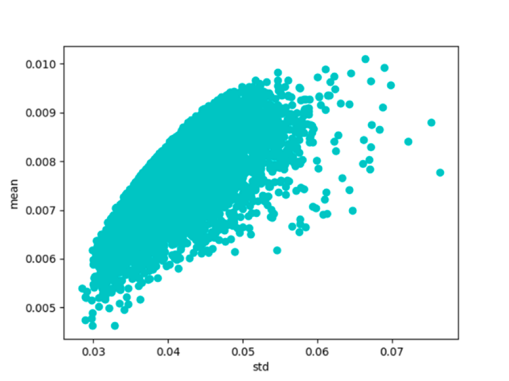
Figure 2: Random portfolios of returns in a mean-variance diagram (source: BSIC)
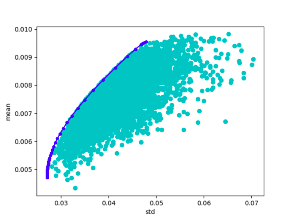
Figure 3: Efficient frontier (source: BSIC)
Here is the covariance matrix between coins over the full time period:
| BTC | ETH | LTC | DASH | XMR | XRP | |
| BTC | 0.0008934 | 0.0003906 | 0.0006145 | 0.0003122 | 0.0003777 | 0.0000625 |
| ETH | 0.0003906 | 0.0061418 | 0.0003878 | 0.0002893 | 0.0006947 | -0.0001177 |
| LTC | 0.0006145 | 0.0003878 | 0.0025754 | 0.0001994 | 0.0003253 | 0.0007965 |
| DASH | 0.0003122 | 0.0002893 | 0.0001994 | 0.0060094 | -0.0002248 | -0.0001462 |
| XMR | 0.0003777 | 0.0006947 | 0.0003253 | -0.0002248 | 0.0109671 | 0.0003300 |
| XRP | 0.0000625 | -0.0001177 | 0.0007965 | -0.0001462 | 0.0003300 | 0.0135399 |
Table 1: Covariance matrix (source: BSIC)
Subsequently we built two portfolios. The first one, ‘Optimized’, was obtained with the following procedure. Every month the algorithm would optimize the weights over the previous two months, rebalance the portfolio and then pause trading for the following 30 days. In the second one, ‘Rebalanced’, the weights were optimized over the previous month and then kept constant for 30 days, meaning that every day there had to be a rebalancing taking into account changes in prices. In each case, the selected weights were those of the global minimum-variance portfolio.
We then compared our portfolios against two passive portfolios: ‘Equal_weights’ with constant equal weights for the whole period and ‘BTC’ invested only in Bitcoin (Figure 4).
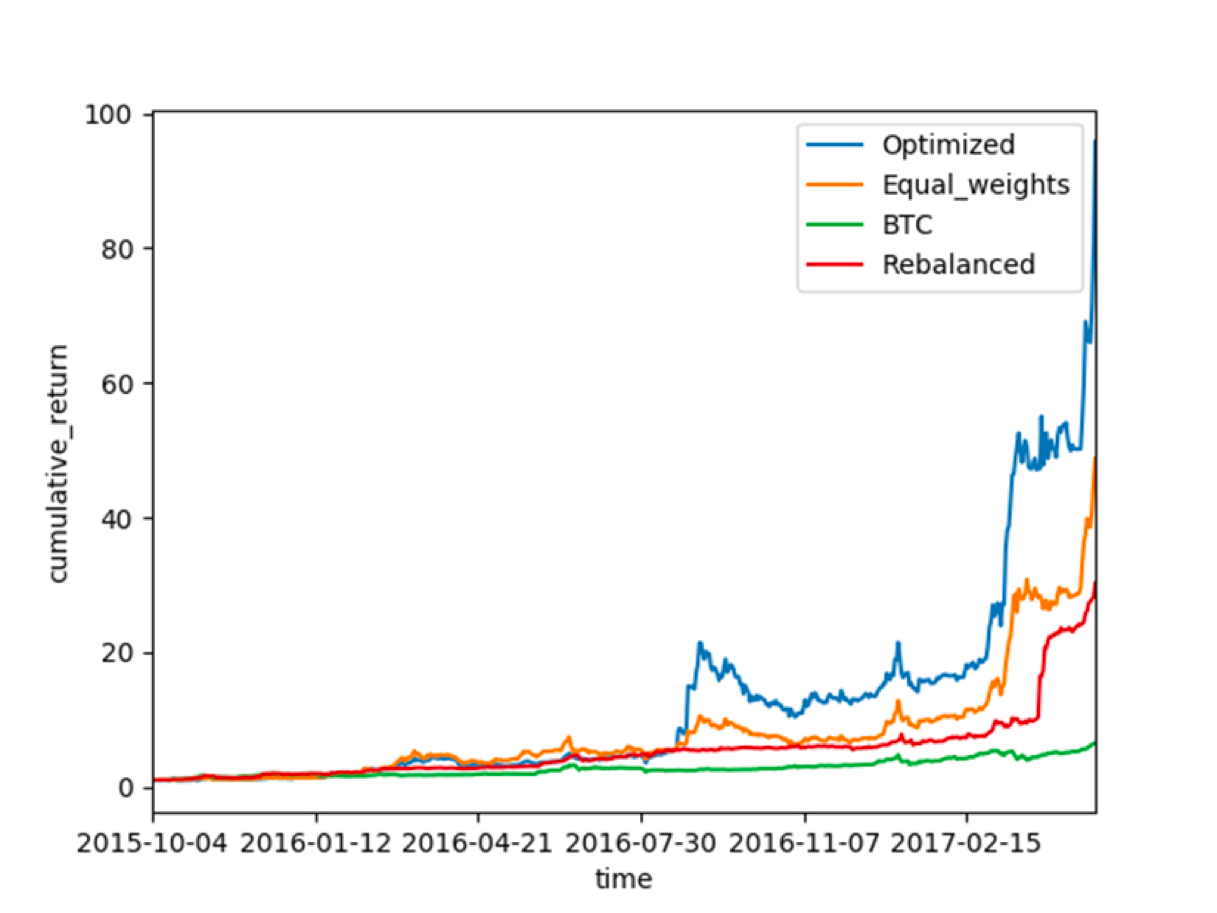
Figure 4: Cumulative return of the 4 strategies (source: BSIC)
Here are some key results of the portfolios:
| Mean return | Std | CV | Cumulative return | |
| Optimized | 0.98603% | 0.0660454 | 6.6981125 | 9581.44292% |
| Equal_weights | 0.79034% | 0.0488792 | 6.1845659 | 4872.99089% |
| BTC | 0.37027% | 0.0304121 | 8.2133935 | 649.10692% |
| Rebalanced | 0.65047% | 0.0370800 | 5.7005283 | 3020.79311% |
Table 2: Performance recap (source: BSIC)
Comment
Consistently with our expectations, ‘Optimized’ beats all the other portfolios at the cost of a greater volatility. This was due to the lack of daily rebalances, which let prices’ volatility influence more the portfolio, especially in the first part of the current year. Conversely, ‘Rebalanced’ showed a lower standard deviation as well as a lower coefficient of variation. Having a daily rebalance meant that single coins volatility were promptly neutralized as to avoid an increase in the coins relative weights. It is worth noting that we assumed no trade commissions: when taken into account, the returns and especially those of ‘Rebalanced’, which requires a high trading activity, might well be lower.
It might be of interest to know that following a recent spike in popularity of altcoins (Figure 5), the Dominance Index, measuring Bitcoin market cap to total market cap of cryptocurrencies, sharply declined: it was well above 90% until the end of 2016, it is now below 60%.
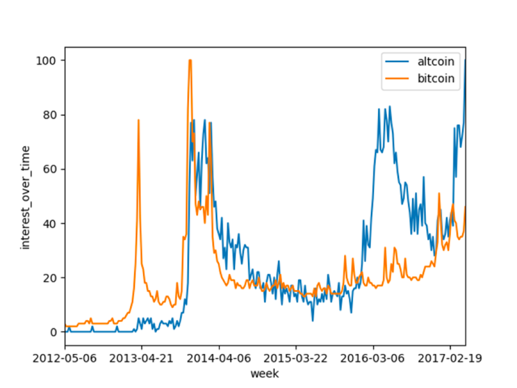
Figure 5: Interest over time (source: Google Trends)


1 Comment
The Importance of Risk Management and Psychology When Trading Crypto – BTC Ethereum Crypto Currency Blog · 17 April 2020 at 15:53
[…] amount of risk. The mathematical framework MPT has been applied by a number of groups. Recent research by the Bocconi Students Investment Club at Bocconi University in Milan showed that applying the […]