Introduction
In this article, we explore how optimising entry and exit points can improve the performance of mean reversion strategies, specifically within a purchasing power parity (PPP) framework. We address this optimisation challenge, by exploring two complementary approaches: a theoretical model-based approach and a numerical method. Due to the simplicity of the intuition behind the approach and their consistency across asset classes, mean reversion strategies are often particularly attractive to investors. However, the success of such strategies depends largely on how accurate of the trading bands, i.e. the entry and exit thresholds, are defined. Accurate calibration is of major importance, as setting these bands too tightly can imply excessive transaction costs due to the multitude of executed trades, while setting them too wide misses valuable opportunities. In this article, we apply an approach proposed by Zeng and Lee (2014) that optimizes entry and exit points on the assumption that deviations from PPP follow a Ornstein-Uhlenbeck (OU) process.
A choice of a linear RV model for currencies: Purchasing Power Parity
Purchasing Power Parity (PPP) is a popular approach to monetary theory that posits that in the long run, currency returns should be driven by cross-country inflation differentials. While the theory provides a compelling rationale for long-term currency valuation, short run FX rates often fluctuate heavily and deviate from PPP predictions. Short-run deviations are very common and are often influenced by factors ranging from market frictions to economic policies such as capital controls. In this article, we explore whether these deviations exhibit mean-reverting behaviour and whether such dynamics can be exploited.
We run PPP regressions on 15 currencies against the U.S. Dollar in the following form:

Where  is the monthly rate of appreciation/depreciation of a currency and
 is its inflation differential with the USD. Since the inflation data we used is monthly, while FX data was provided on a daily basis, we make monthly predictions every time a new inflation data point becomes available, and during the month we measure dislocations in the daily FX rate from that month’s prediction. While PPP is conventionally a long-run theory, we chose a window of 1 month to measure returns and inflation differentials because we discovered that longer windows (e.g. 1 year) would slow down reversion speeds and make relative value trading less attractive.
A common approach is to then normalize the residuals by demeaning and standardizing them, before generating signals. We instead chose to create the signal-generating series by transforming the residuals with a sigmoid function (in our case,  ) to scale the data in the interval
 ![[-1,1]](https://bsic.it/wp-content/ql-cache/quicklatex.com-311be99e99eac21772cd1920278c092b_l3.png "Rendered by QuickLaTeX.com") and to ensure that extreme values do not overinfluence trading decisions.
and to ensure that extreme values do not overinfluence trading decisions.
Next, we’ll explore the approach proposed by Zeng and Lee (2014) and how we implemented it practically.
Analytical determination of optimal Entry and Exit points
Lin and Barziy (2021) rightly point out the two core challenges in developing a pairs trading strategy. The first is identifying which assets to pair in order to form a process exhibiting mean-reverting behavior. The second is determining when to trade – essentially, how to select optimal entry and exit points for the strategy.
Traditionally, these entry and exit decisions are made by defining thresholds tied to the standard deviation of the spread or dislocation between asset prices. A trade is triggered when the spread hits a multiple of its standard deviation, with the proportionality constant typically found through empirical optimization. This optimization usually targets either the total return of the strategy or its Sharpe ratio.
The approach taken in the Hudson paper by Lin and Barziy (2021) deviates from this empirical framework, aligning instead with the theoretical methods introduced by Bertram (2010) for long-only strategies and extended by Zeng and Lee (2014) to allow for both long and short positions. Rather than relying on backtested parameter fitting, this line of work seeks to analytically optimize the expected return per unit of time.
Assuming the price spread between the paired assets follows an exponential Ornstein-Uhlenbeck process, the problem is reframed in terms of the first-passage time of the process. This makes it possible to derive closed-form expressions for the expected trade duration, its variance, the expected return per unit of time, and the variance of that return. Based on these results, optimal trading thresholds can then be determined by maximizing either the expected return or the Sharpe ratio.
The key is to consider the entire trading cycle—from entry to exit—as a first-passage event of a mean-reverting process hitting a two-sided boundary. Using the parameters of the OU process, expressions for expected returns and variances are derived and subsequently optimized. The analytical tractability of the problem is enhanced by switching to dimensionless variables, which simplifies the resulting equations. In the end, one obtains a polynomial equation of infinite (but decaying) degree, which must be solved and then transformed back into dimensional terms using the original OU parameters.
When searching for an exit point  for a trade between 0 and its entry point
  , with transaction costs
  the maximisation problem solved in Zeng and Lee (2014) is the following:


Once they show that  for any , they then set
  to find
  through the following equation:

They then optimize the same  for
for  . The optimization problem is the same, but with a different constraint:


Where they show that the for the gradient of to be zero, the only solution can only be  , so that
  . They then solve the following equation for :

The authors also show that the second maximisation problem always yields greater maximal returns than the first, when transaction costs are present. We implemented a root-finding solver for the largest terminal sum index that we could find that wouldn’t result in computing errors.
One of the key findings of Zeng and Lee (2014) is that under the above-mentioned assumptions, when transaction costs are non-zero, the optimal exit points for a long (short) trade should not be set to the long-run mean of the series, but rather to the optimal short (long) entry points, thus allowing for no waiting time between trades.
Estimation of Ornstein-Uhlenbeck parameters
When implementing this particular approach with respect to our PPP strategy, we estimate OU parameters on PPP dislocations from the first half of the data. Specifically, we require  in order to adapt the optimized result to the nature of our dislocations. An OU process is of the form:

To derive these parameters with respect to the dislocations we’ve observed on our PPP strategy, we can use OLS on a discretized OU process. Alternatively, as other papers have employed in past parameter estimations, MLE is a suitable candidate. However, the computation of this estimation approach is much more computationally expensive, and given standard properties of the log likelihood function, MLE and OLS should theoretically produce equivalent parameter estimates due to the Markov property of OU processes.
When performing OLS, we take a discretized version of our OU, based on the exact solution of its SDE:

Discretizing the OU process into, essentially, an AR(1) process is useful because it allows us to use OLS to estimate the  and
and  terms, which can then be plugged back into the standard OU using the following relations:


Now, how do we apply this method in such a way which avoids forward-looking bias? Simple: we take an expanding sample of the dislocations and re-adjust the parameters for our OU at each particular time-step (in our case, days). You might be wondering: “Is there a specific reason we prefer an expanding approach to a rolling one in this instance?” And, in fact, the answer is yes. Using an expanding sample is quite useful when you don’t expect the nature of your process’ parameters to change dramatically through time, which is different from something like a rolling window, which assumes that older datapoints are irrelevant to future forecasts. Since we believe the former assumption to hold true, the more datapoints, the merrier.
Results and Findings
We run the above-mentioned procedures on 16 years of data from 2008 to 2024 on AUD, BRL, CAD, CLP, CNY, DKK, EUR, GBP, ILS, JPY, KRW, MXN, MYR, NOK and NZD. We calibrate optimal entry/exit points only once at the end of the first half of the data (the train set) and apply those optimal bands to the rest of the data (the test set). More frequent calibration of optimal entry/exit points could be an interesting subject for expansion of this article.
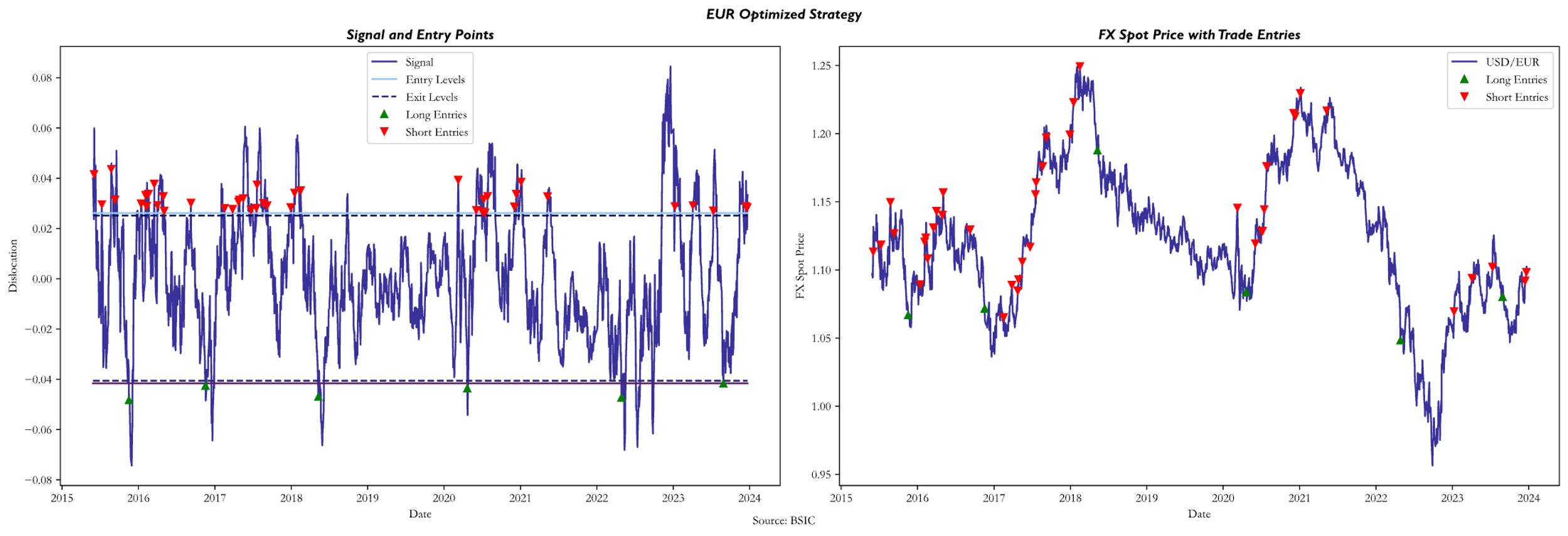
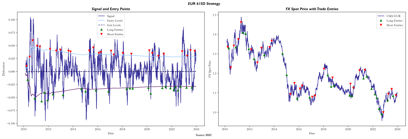
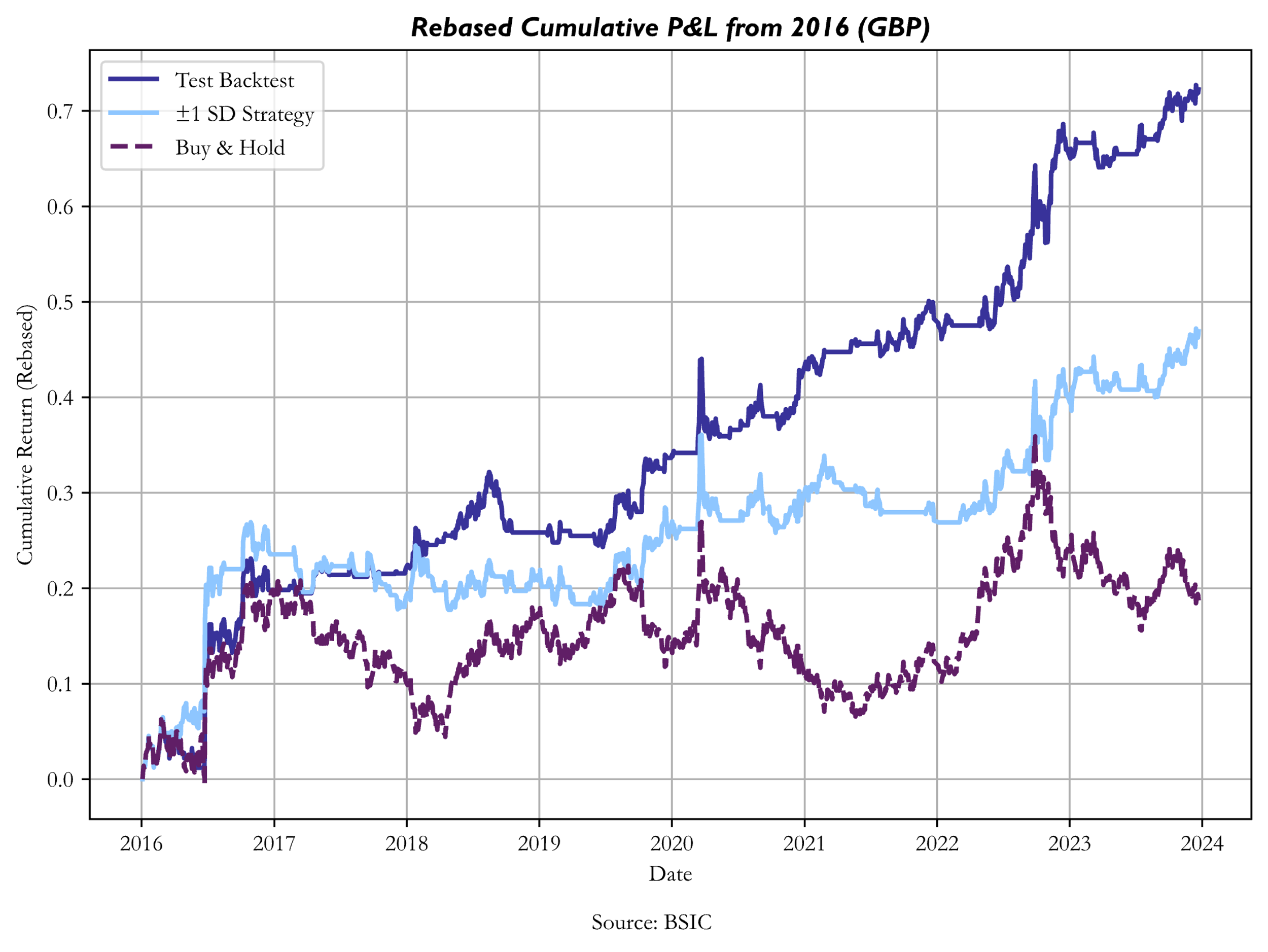
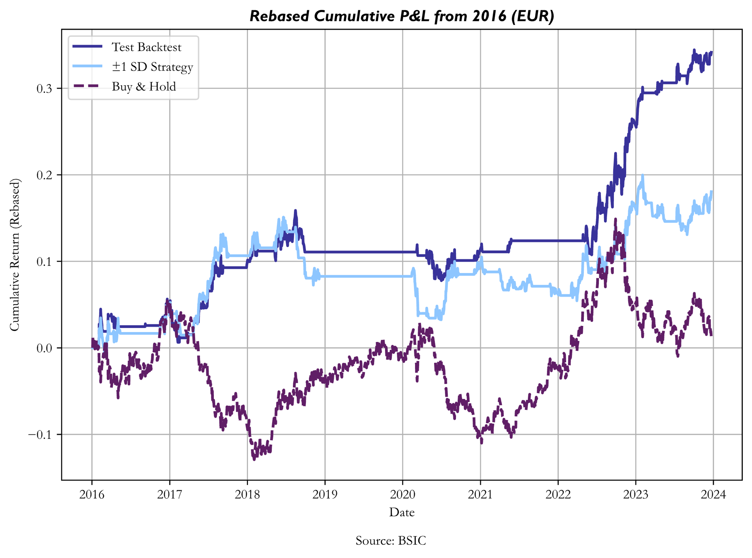
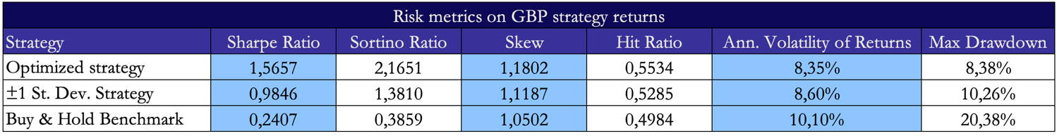
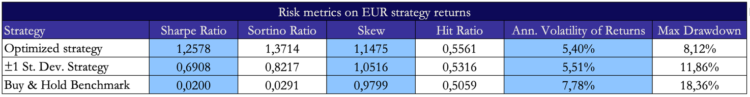
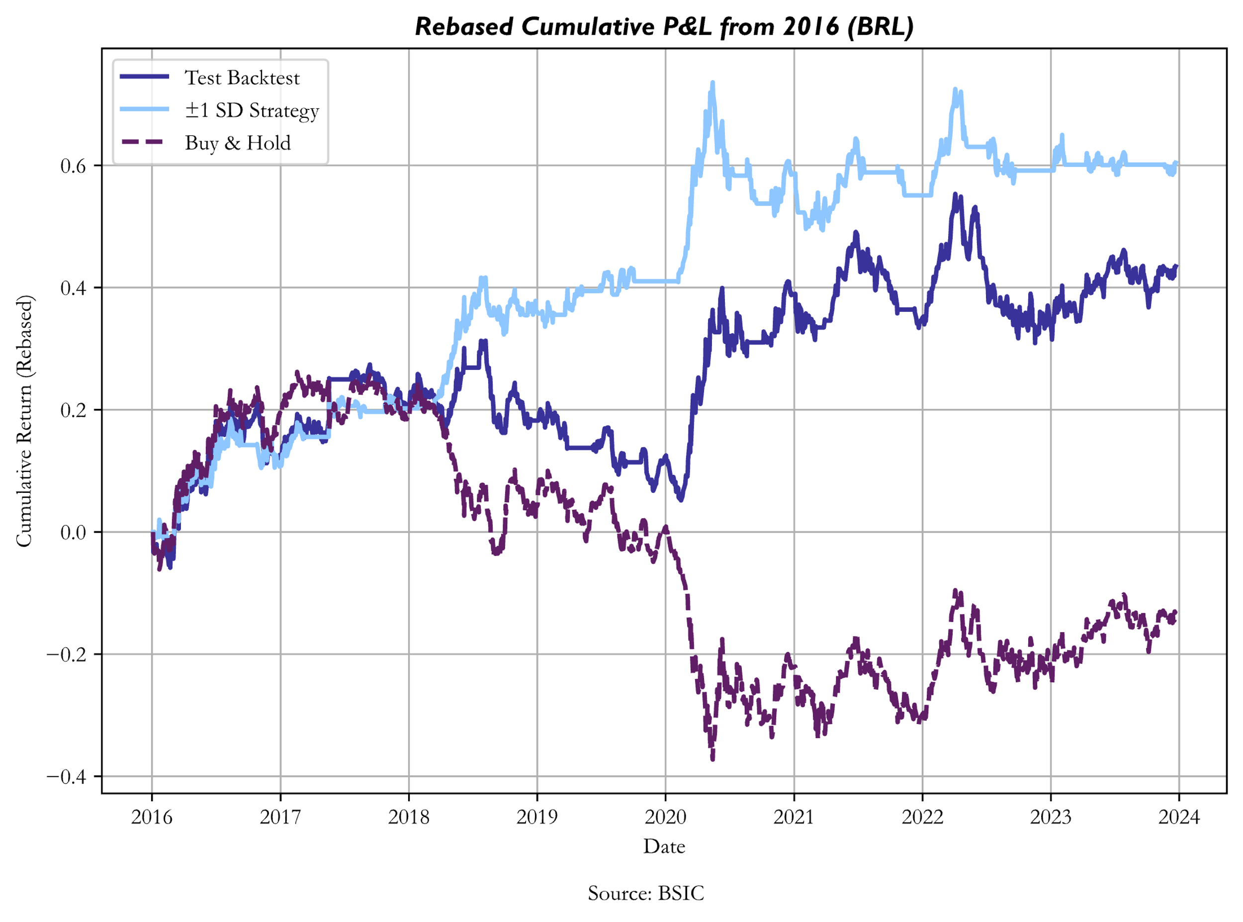
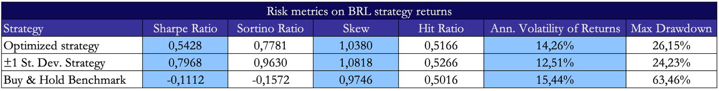
The main subject of interest of the article isn’t whether the PPP strategy produces excess returns compared to a benchmark, but rather whether the optimal calibration of entry/exit points produces greater profits compared to an arbitrarily set trading rule. As a benchmark, we chose to display the performance of trading dislocations with a +1/-1 expanding standard deviation rule to avoid forward-looking bias. The arbitrary trading rule functions as follows: when the transformed dislocation series is at least one standard deviation below (above) its mean, a long (short) signal is generated; positions are cleared when the transformed dislocation series crosses its mean.
Source: BSIC
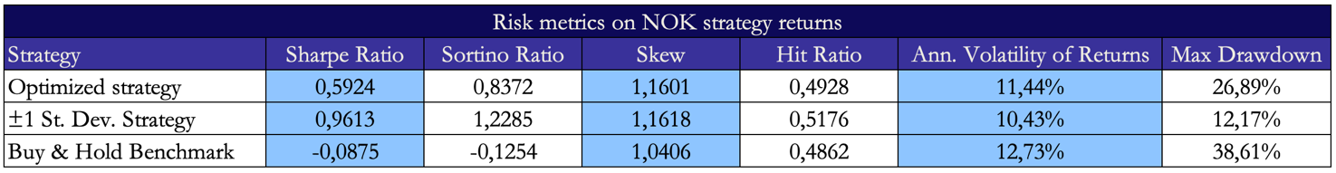
The optimized strategy outperformed (both in terms of Sharpe Ratio and Cumulative Returns) the arbitrary trading rule on the test set on all currencies except CAD, DKK, ILS, KRW, MYR and NOK. A factor that seems to have driven the underperformance of the optimized strategy when trading these 6 currencies against the dollar is linked to non-stationarity of the signal series. In particular, it seems that mean hitting times for trades on these 6 currencies against the USD were somewhat different between train set and test set data. This implies that the OLS parameters that were estimated on the train set caused the optimization process to return relatively wide trading bands, and in a test set with slower mean reversions, a set of relatively tighter trading bands would have been preferrable. Conversely, where mean reversion speeds were greater in the test set than they were in the train set, it could’ve been preferrable to implement a wider pair of bands, to avoid incurring into excessive transaction costs and benefitting from larger swings.
With certain currencies (especially DKK) we also encountered volatility differences in the signal series between the train set and the test set. When trading bands are fine-tuned to a train set series that is more volatile than the test set one, they tend to be wider, thus decreasing the number of trades as well as increasing position holding times. Conversely, when the signal-generating series tends to be less volatile in the train set data than in the test set data, more signals are generated, but without capturing larger swings, and incremental transaction costs potentially outweigh incremental profits.
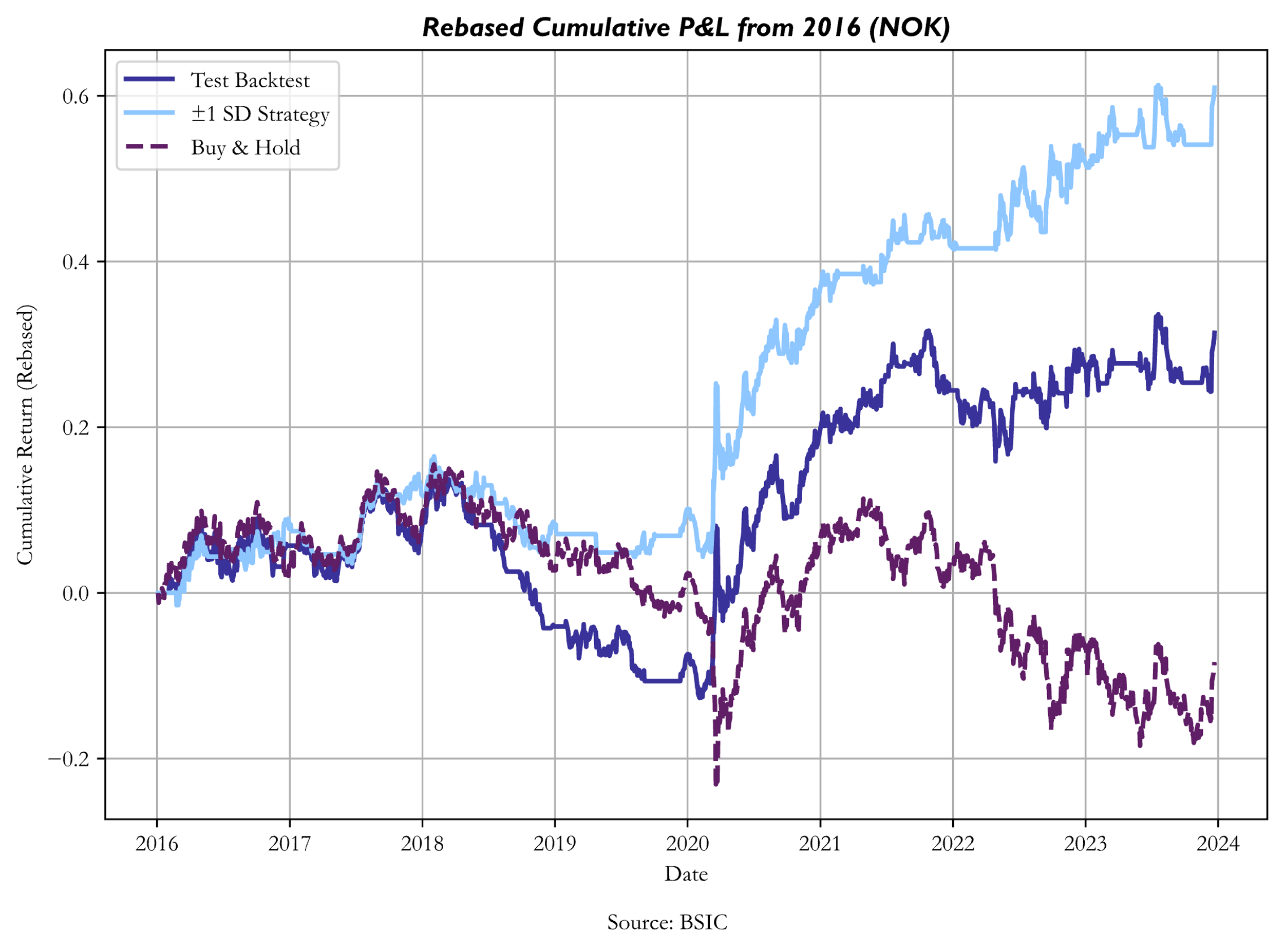
Source: BSIC
Conclusions and Final Remarks
Our investigations should serve as a first approach to the subject of determining optimal entry and exit points. Further experiments could (and should) be conducted. A first result is that a rule of thumb does not always perform as well as it sounds. The second key result is that the data points in favour of the presented approach being a generally valid one, but with potential for fallacies due to the underlying assumptions on the signal series.
We identified signs that OU parameters may not be stable for very long periods of time (hence volatility and mean reversion speed regime shifts), which could be dealt with by either implementing dynamic drift and diffusion models, or by changing the way in which OLS parameters are estimated (more frequently and/or on shorter timespans). Additionally, since the focus of the article is to present this method as a general approach to RV trading across asset classes, we should also consider that a specific parametric form (as the OU form we imposed) might not be the best fit for all mean-reverting signal series. Experimenting with nonparametric calibration of drift and diffusion coefficients could be a way to tackle the problem. Alternatively, numerical approaches that optimize bands directly on the observed data by maximizing could also be interesting to investigate, if not too computationally expensive.
Lastly, we also suggest that – provided that a solid parameter estimator and model specification be found for the signal series – a Monte Carlo simulation of signal paths could be useful to test the validity of estimated bands, by computing returns on each of those paths using the bands estimated in-sample. This, along with the previously mentioned suggestions on further areas of investigation, provides a decent amount of content to further investigate in the future.
Appendix: Risk Metrics for other currency pairs
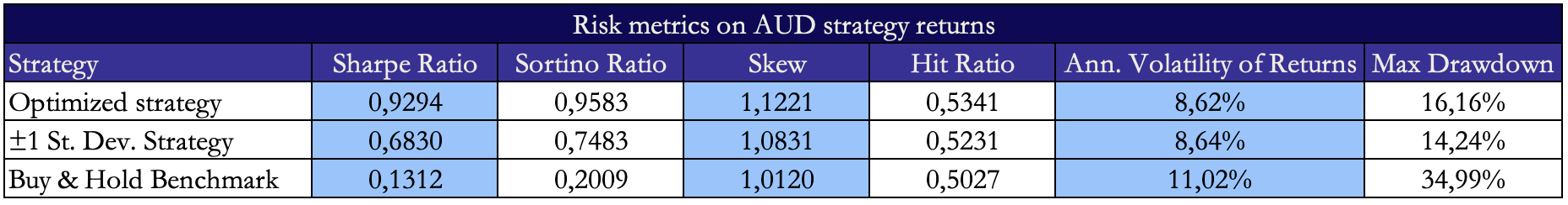

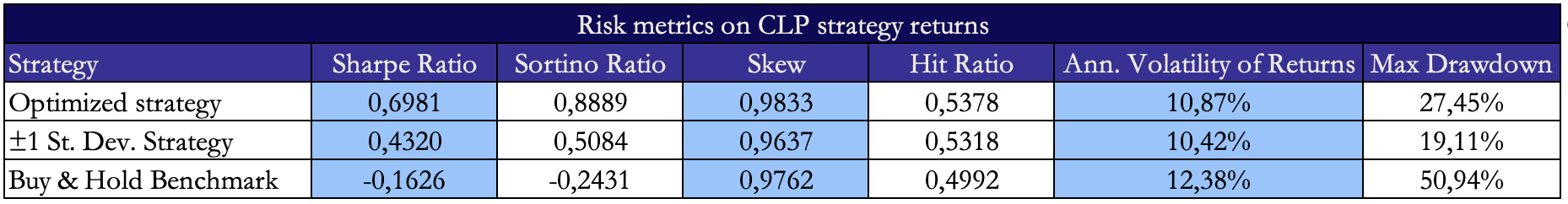
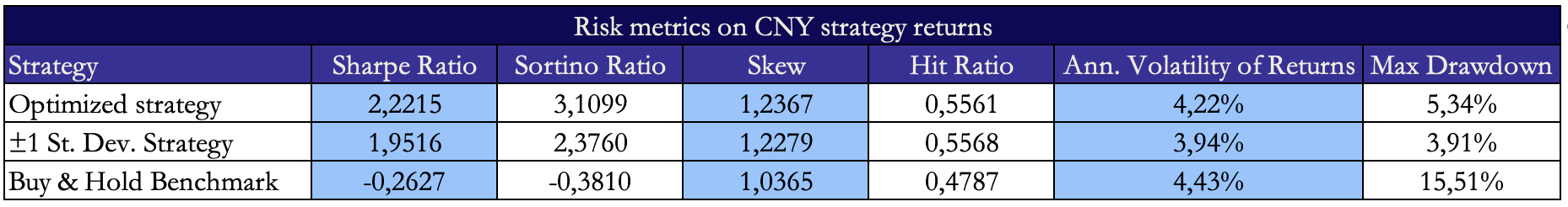
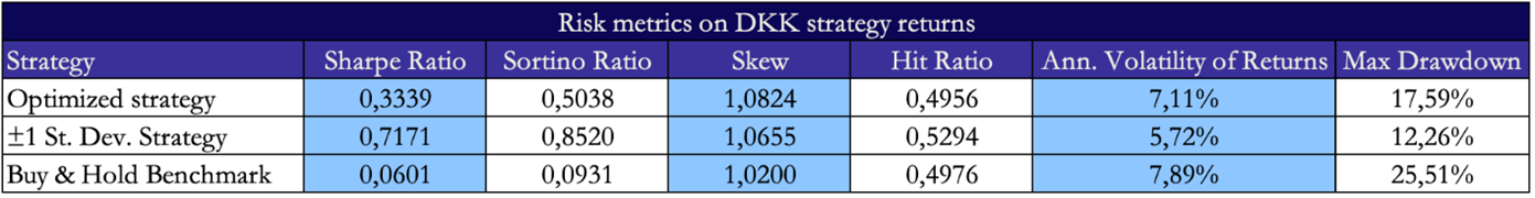
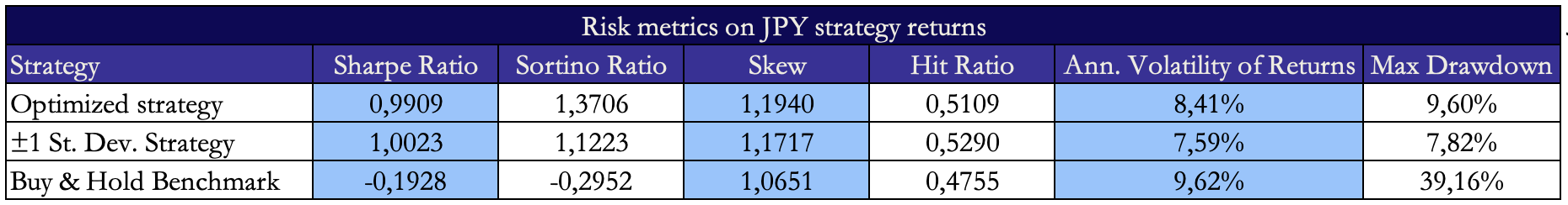
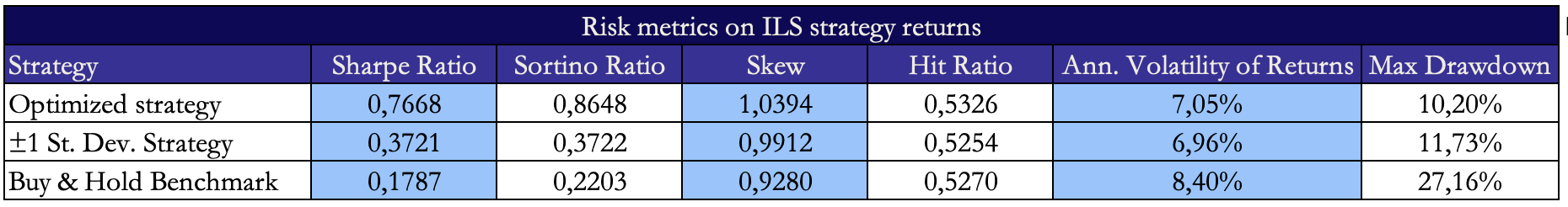
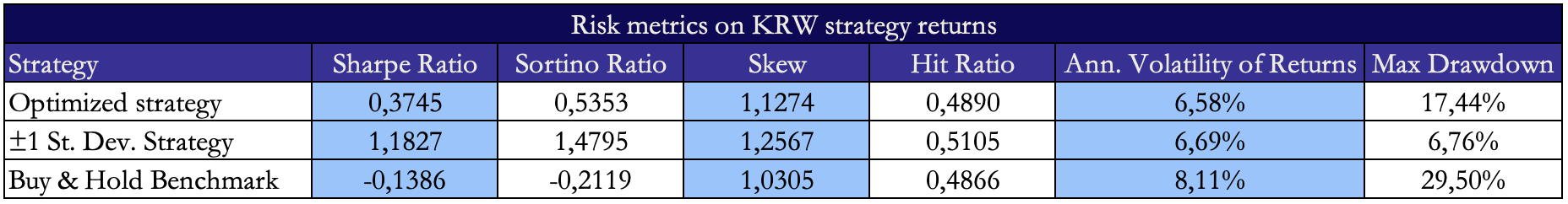

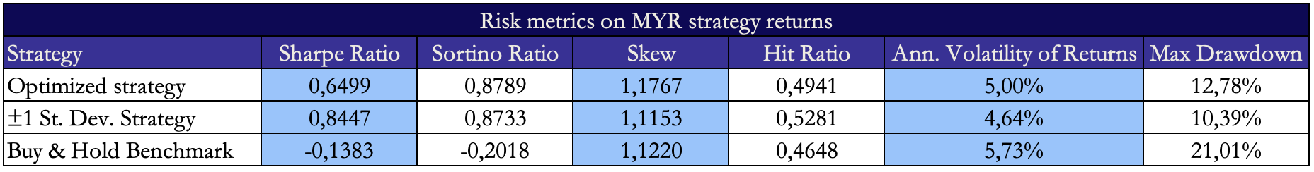
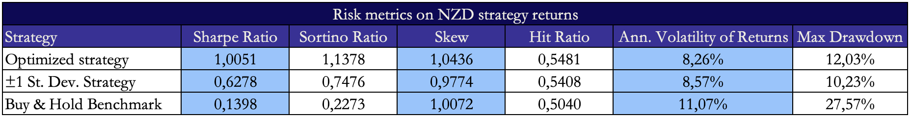
Source: BSIC
References
[1] Zeng, Z. & Lee, C. “Pairs trading: optimal thresholds and profitability”, 2014
[2] Lin, A. & Barziy, I. “Optimal Trading Thresholds for the O-U Process”, 2021
[3] Bertram, W. K. “Analytic solutions for optimal statistical arbitrage trading”, 2010


0 Comments