Introduction
Statistical arbitrage is a class of trading strategies that profit from exploiting what are believed to be market inefficiencies. These inefficiencies are determined through statistical and econometric techniques. Note that the arbitrage part should by no means suggest a riskless strategy, rather a strategy in which risk is statistically assessed.
One of the earliest and simplest types of statistical arbitrage is pairs trading. In short, pairs trading is a strategy in which two securities that have been cointegrated over the years are identified and short-term deviation from their long-term equilibrium creates trading opportunities.
In this article, we show how to build a backtesting environment with Python, which you can find in this GitHub repository. For a more extensive explanation of pairs trading please refer to this article. Before diving into the implementation of the code, it is important to deeply understand how to test a hypothetical statistical relationship. To do that, we recall the concepts of stationarity, correlation and cointegration.
A stationary process is characterized by constant mean, variance and autocorrelation. Nonstationary time series do not have the tendency to revert to their mean and vice versa.
Correlation is a measure of the linear relationship between stationary variables. As a consequence, when dealing with non-stationary variables, correlation is often spurious. For this reason, it is good practice to avoid calculating correlation coefficients or regressing two non-stationary processes. However, most of the processes that we deal with in the real world are non-stationary. This leads to the necessity to study them despite some imperfections.
To do this, cointegration comes into play. Suppose two time series X and Y are non-stationary and integrated of order d, then they are cointegrated if it is possible to find a linear combination  that is integrated of order less than d. In our case, if two securities are non-stationary time series of order 1 and if a linear combination between two securities (spread) is tested to be integrated of order 0, in other words stationary, then we define the two securities as cointegrated.
While the order of integration is usually tested through the Augmented Dickey-Fuller test, to test cointegration Engle-Granger seems the perfect choice. After having determined a certain coefficient  by regressing X on Y, the residuals (spread) are tested for stationarity through an Augmented Dickey-Fuller test. In simple terms, the Dickey-Fuller test is a procedure in which the coefficient of an autoregressive process is tested for its significance. If the coefficient is 1, the process is a random walk and the unit root (non-stationarity) cannot be rejected. On the other hand, if the coefficient is significantly less than 1, then the unit root is rejected and the process is considered to be stationary.
To summarize, cointegration implies that the variables share similar stochastic trends, and therefore their residuals follow a stationary process. Two cointegrated variables may not necessarily move in the same direction (correlation), but the distance between them will remain constant over time.
Moreover, in selecting our pairs, we will also consider the Hurst exponent, which measures the long-term memory of time series. By identifying the persistence of trends, it distinguishes random from non-random systems. A value between 0.5 and 1 indicates persistent behavior (positive autocorrelation – trend). A value between 0 and 0.5 indicates an anti-persistent behavior (negative autocorrelation – mean reversion) and a value of 0.5 indicates a true random process (Brownian time series). The exponent is calculated using the so-called Rescaled Range analysis, but we will not go through its computation due to the numerous steps required.
The code
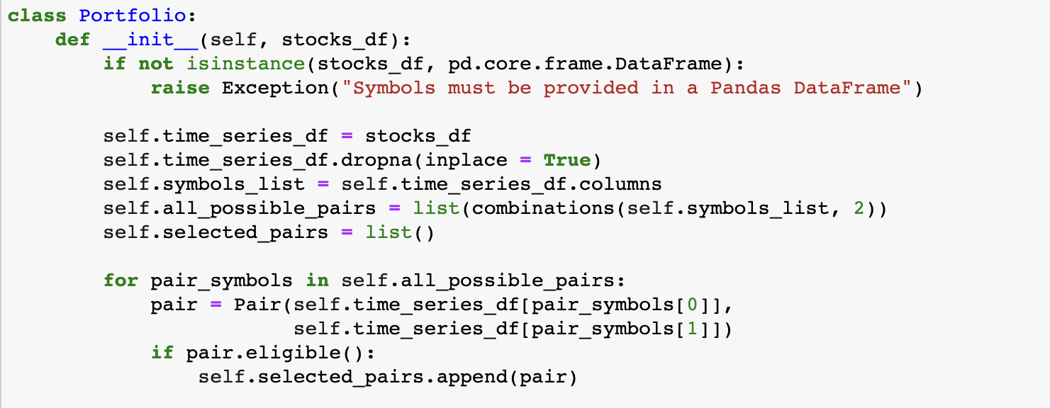
The two main classes are Portfolio and Pair. The former receives the stocks dataframe as input and generates all the possible pairs combinations via itertools.combinations. After doing that, a for loop goes through all the possible pairs and, for each of them, it creates a Pair object.
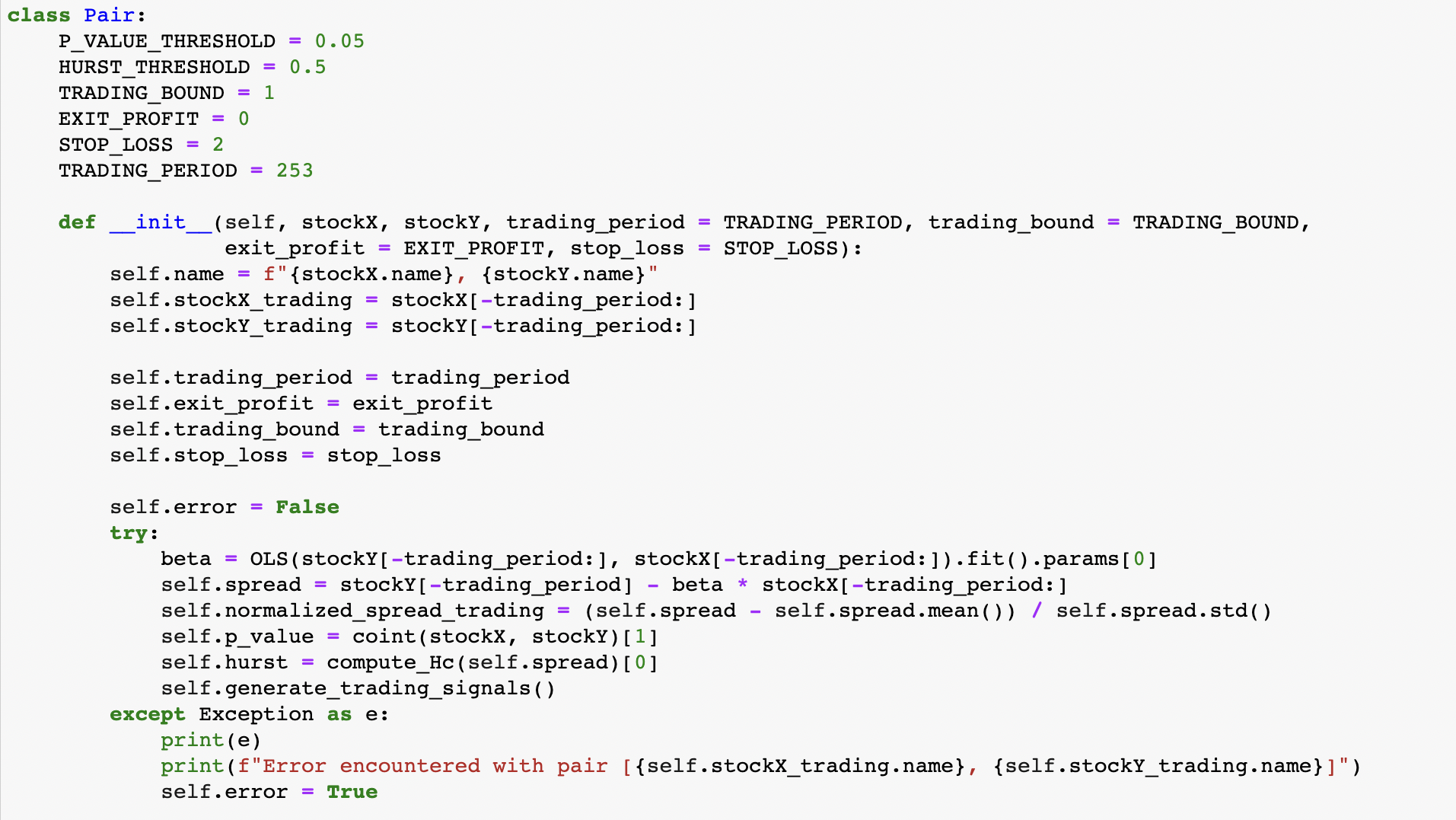
When a Pair object is created, an OLS is performed between the two stocks, and its Beta is used to compute the spread between the two securities. In addition to this, the spread is normalized and the p-value of Engle-Granger test and the Hurst Exponent of the spread are computed.
These two values are then used in the Pair.eligible method, in which the pairs are tested for eligibility. In particular, the default thresholds are set respectively to 0.05 and 0.5, but they can be modified by the end user. This means that, for a pair in order to be eligible, it must have a p-value smaller than 0.05 and a Hurst exponent smaller than 0.5. This method is then used in the Portfolio class in order to check which pairs are going to be included in the selected_pairs list, on which the trading strategy will be applied.

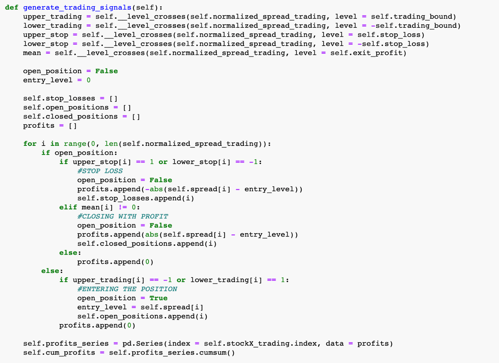
Finally, the method plot_pair shows a plot of the normalized spread of a pair, as well as the price of the two securities and, most importantly, the trading signals adopted by the trading strategy.
Trading strategy
Once all the pairs have been filtered out from the initial stocks, a pairs trading strategy should be defined. This consists primarily in setting the trading period, as well as the thresholds at which to enter a position and to exit from it, either with a profit or by incurring in a stop loss. In this case, all these thresholds are directly set in the constructor of the Pair class, and they always refer to the normalized spread between the two securities. Their default values are the following:
- Trading period: 253 days;
- Entry point: 1 std;
- Exit point: 0 std;
- Stop Loss: 2 std.
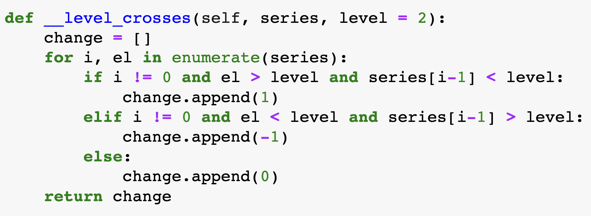
In order to detect when the spread crosses a certain threshold, the __level_crosses method is used, but we won’t go into the details of this. To understand how the strategy works, let’s have a look at this pair:
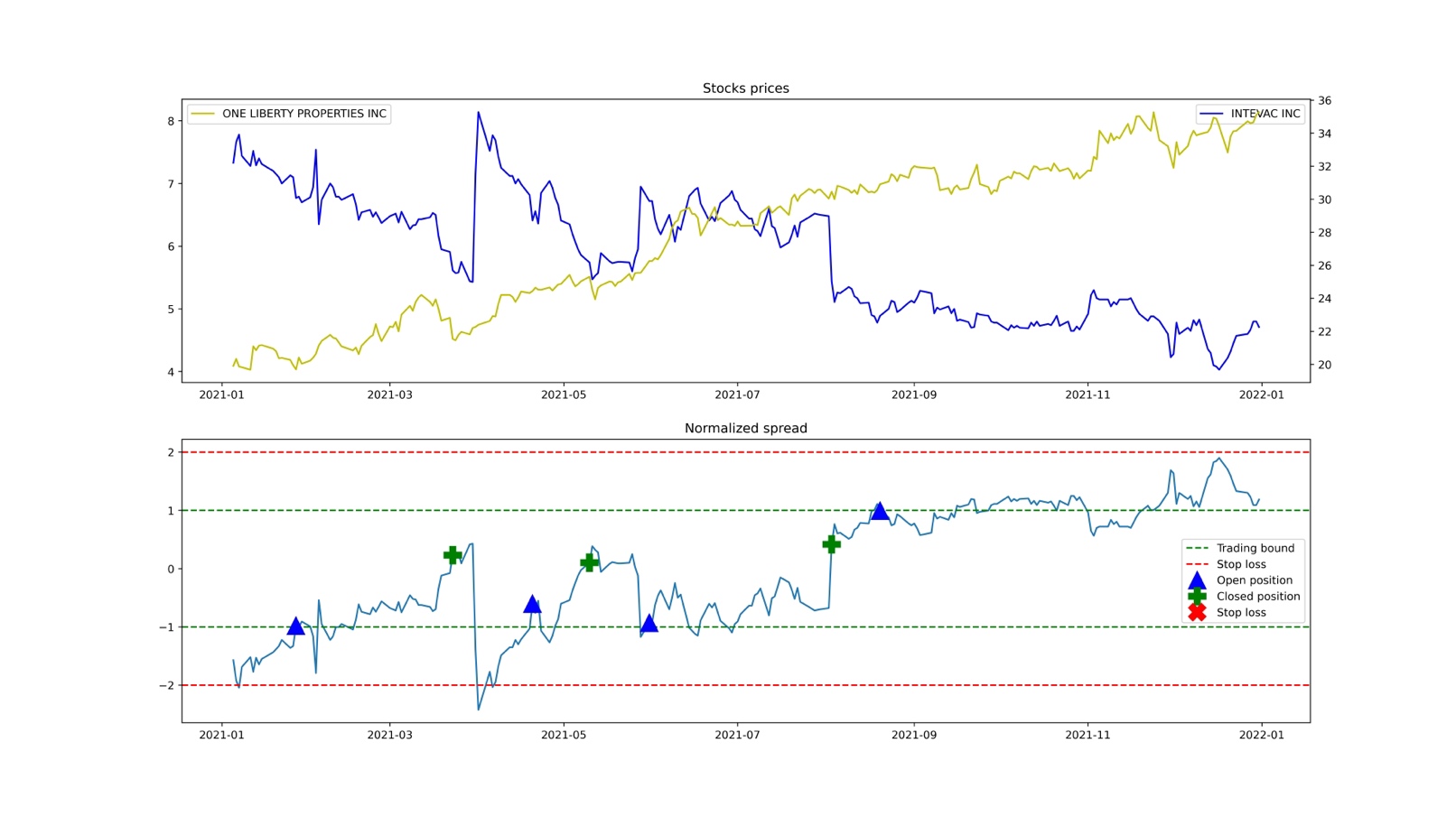
Source: BSIC
Entry points, exit points and stop losses are represented by blue triangles, green plus signs and red crosses.
As it has been already mentioned, the strategy is based on the assumption that short-term deviations from the long-term equilibrium of the two securities create trading opportunities, and for this reason we enter in a position whenever the normalized spread diverges more than a certain amount, which is depicted by the dotted green lines. But what do we exactly do when entering a position? Recall the spread formula:
If the spread is too high (above 1std) it means that Y is the rich leg (overvalued) to short and X is the cheap leg on which to go long. If the spread is too low (below 1std) we do the exact opposite.
We close the position as soon as the spread gets back to its normal level, id est when it reaches the Exit Point threshold. Alternatively, if the spread diverges to an excessive extent, which is set by default to 2 std, we incur in a stop loss. We set the stop loss so as to prevent exogenous shocks from causing huge losses.
Since every trade consists in both a long position and a short position, these positions can be considered entirely or at least partially self-financing. Indeed, the capital raised from selling a stock will be reinvested in buying the other stock. The computation of returns on zero-cost portfolios is a problematic concept and different solutions have been proposed to overcome this problem: returns may be calculated only on the long leg of the position, on the sum of the long leg and the absolute value of the short leg of the position or may take in consideration the margin capital needed to undertake the short position.
As returns can vary significantly according to the method chosen, in our backtesting environment we preferred to keep them as a simple difference between closing and initial spread. A less sensitive parameter that might be useful to evaluate the performance of the strategy is the percentage of profitable trades.
How to test the code with your data
In order to feed the program with stocks data, we have downloaded the CRSP Daily Stock database, with a date range from 01/01/2000 to 31/12/2021. However, the end user can adopt whatever stocks database he/she prefers, as long as it is similar to the following structure:
- Each column corresponds to a certain company, and each row to all the observations on a certain date.
- NaN values should be interpolated, if present.
- Prices columns should be made of nonnegative entries: for instance CRSP Daily Stock uses negative sign as a convention for when the closing price is not available on any given trading day.
Here’s an example of how the database should look like after going through these preprocessing procedures:
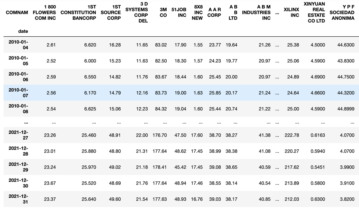
Source: BSIC
Future improvements
As we have shown, in order to select the eligible pairs from a portfolio of n stocks, it’s necessary to find out all the possible combinations of stocks, which are exactly  , and for each combination we perform a linear regression, so as to calculate , as well as a few statistical tests, namely, the Engle-Granger test and the calculation of the Hurst exponent. We can quickly see of this becomes infeasible as n grows. For instance, if
  , the number of iterations is in the vicinity of 4.5 mln, which is quite computationally heavy for a standard computer.
For this reason, various Machine Learning techniques have been adopted in the last few years (see Han, He, Toh 2021). In particular, clustering algorithms manage to discover all the eligible pairs without confronting each stock pairwise. What’s even more, it’s possible to embed in the input of the algorithm not only past price data, like with the cointegration approach, but firm characteristics as well, and by doing this the Sharpe ratio of the selected portfolio increases sensibly.


3 Comments
Joseph E Farrell · 7 August 2022 at 5:47
I have a strategy that i constructed and amazingly similar to yours. Are you able to discuss your execution and compare results?
Luca · 17 November 2022 at 14:52
Mi spiace ma questa implementazione è ricca di errori. A parte i refusi nel codice la cosa più eclatante è che è implementato ricavando i parametri di controllo sulla zona poi sottoposta a test. Ciò naturalmente implica che il futuro sia noto…. probabilmente è sfuggito qualcosa nel codice… suggerisco una revisione. Comunque al netto di questo l’idea, soprattutto per la sua semplicità, è interessante.
Simple Portfolio Pairs Cointegration Test – Jed Gore · 22 February 2023 at 20:30
[…] Good article on this topic here: https://bsic.it/pairs-trading-building-a-backtesting-environment-with-python/ […]