Risk Neutral Density Estimation from Option Prices

Introduction

Options are among the most information-rich instruments in financial markets. Unlike traditional asset classes, such as equities or bonds, whose prices reflect a single point estimate of value, options are priced across a continuum of strikes and maturities, which means they embed an entire probability distribution over future underlying asset price. This distribution, known as the risk-neutral distribution, sits at the heart of modern quantitative finance and derivative pricing theory.

In a complete, arbitrage-free market, the 1st and 2nd fundamental theorems of asset pricing guarantee the existence of a unique probability measure, the risk-neutral measure $\mathbb{Q}$ , under which the discounted price of any traded asset follows a martingale. Formally, for any security with payoff $X_{T}$ at maturity $T$ , its time- $t$ price satisfies:

$V_{t} = e^{-r(T-t)} E_{t}^{\mathbb{Q}}\left[V_{T}\right] = e^{-r(T-t)} E^{\mathbb{Q}}\left[V_{T} \mid \mathcal{F}_{t}\right]$

Where $r$ is the risk-free rate and $\mathcal{F}_{t}$ denotes the information set available at time $t$ . Under this measure, all assets are expected to grow at the risk-free rate, regardless of their actual risk profile. In simple terms, the martingale condition ensures that the best forecast you can make of an asset value in the future is simply the properly capitalized price you are currently observing in the market.

A critical point to make is that the risk-neutral probability measure $\mathbb{Q}$ is different from the real-world probability measure $\mathbb{P}$ , under which investors price risk and demand compensation for bearing uncertainty. Nonetheless, the two probability measures are related; therefore, even if $\mathbb{Q}$ does not represent the market’s true probabilistic beliefs about the future, it still remains deeply informative. Specifically, we lose information about the expected returns of the markets, since expected returns under $\mathbb{Q}$ over one year are all equal to the risk-free rate $r$ , but it carries the consensus view on uncertainty, directional asymmetry and tail risk through the second, third, and fourth standardized moments: variance, skewness, and kurtosis

In this article, we show how to extract the risk-neutral density from option prices using Breeden–Litzenberger (1978) result [1], which links the second derivative of call prices with respect to strike to the probability density of the future asset price.

Theoretical Background

The key result of Breeden–Litzenberger is the celebrated identity

$q(K) = e^{rT} \frac{\partial^{2}C}{\partial K^{2}}(K)$

which means that the risk-neutral density at strike $K$ is equal to the second partial derivative of the call price with respect to strike $K$ , multiplied by the capitalization factor $e^{rT}$ . The beauty and elegance of this derivation is that it is not reliant on any pricing model, so it holds for any stochastic process the underlying may follow.

The derivation is not actually too involved, so we derive it for completeness. First ingredient is the Leibniz Rule, which allows us to differentiate an integral with a variable lower limit. Formally, it states that

If $F(K) = \int_{K}^{\infty} g\!\left(S_{T}\right) dS_{T}$ $\Rightarrow$ $\frac{dF(K)}{dK} = -g(K)$

At this point, starting from the general theoretical framework for pricing european derivatives under no-arbitrage, we can derive the celebrated identity

$C(K) = e^{-rT} E^{\mathbb{Q}}\!\left[\left(S_{T}-K\right)^{+}\right] = e^{-rT}\!\int_{0}^{\infty}\!\left(S_{T}-K\right)^{+} q\!\left(S_{T}\right)dS_{T} = e^{-rT}\!\int_{K}^{\infty}\!\left(S_{T}-K\right) q\!\left(S_{T}\right)dS_{T} =$

$= e^{-rT}\!\left[\int_{K}^{\infty} S_{T}\, q\!\left(S_{T}\right)dS_{T} - K\int_{K}^{\infty} q\!\left(S_{T}\right)dS_{T}\right]$

Taking the first partial derivative and exploiting Leibniz Rule

$\frac{\partial C}{\partial K}(K) = e^{-rT}\!\left[-K\,q(K) - \int_{K}^{\infty} q\!\left(S_{T}\right)dS_{T} + K\,q(K)\right] = -e^{-rT}\!\int_{K}^{\infty} q\!\left(S_{T}\right)dS_{T} = -e^{-rT}\,\mathbb{Q}\!\left[S_{T} > K\right]$

Following with the second partial derivative we get Breeden–Litzenberger identity

$\frac{\partial^{2}C}{\partial K^{2}}(K) = \frac{\partial}{\partial K}\!\left[-e^{-rT}\int_{K}^{\infty} q\!\left(S_{T}\right)dS_{T}\right] = -e^{-rT}\!\left[-q(K)\right] = e^{-rT}\,q(K)$

Breeden–Litzenberger approximation

The first problem that emerges from the theoretical part is that in real life there is not a continuum of strike prices for options, but strikes are actually at discrete intervals. The idea is to approximate the second derivative using four call options over 3 consecutive strikes, which build a well-known option spread which is known as a long butterfly:

$\frac{\partial^{2}C}{\partial K^{2}} \approx \frac{C(K-\Delta K) - 2C(K) + C(K+\Delta K)}{\Delta K^{2}} = \frac{\mathrm{Butterfly}(K)}{\Delta K^{2}}$

Which comes directly from summing two Taylor expansions

$C(K+\Delta K) = C(K) + \frac{\partial C}{\partial K}\Delta K + \frac{1}{2}\frac{\partial^{2}C}{\partial K^{2}}\Delta K^{2} + o\!\left(\Delta K^{3}\right)$

$C(K-\Delta K) = C(K) - \frac{\partial C}{\partial K}\Delta K + \frac{1}{2}\frac{\partial^{2}C}{\partial K^{2}}\Delta K^{2} + o\!\left(\Delta K^{3}\right)$

$C(K+\Delta K) + C(K-\Delta K) = 2C(K) + \frac{\partial^{2}C}{\partial K^{2}}\Delta K^{2} + o\!\left(\Delta K^{3}\right)$

$\frac{\partial^{2}C}{\partial K^{2}} \approx \frac{C(K-\Delta K) - 2C(K) + C(K+\Delta K)}{\Delta K^{2}} = \frac{\mathrm{Butterfly}(K)}{\Delta K^{2}}$

Empirical implementation

Armed with the Breeden–Litzenberger identity, we now turn to its application on real market data. The dataset from the OptionMetrics database consists of S&P 500 call option prices spanning 2015–2025, enriched with the corresponding underlying price, risk-free rate, time to maturity, and implied volatility for each (date, expiry) pair.

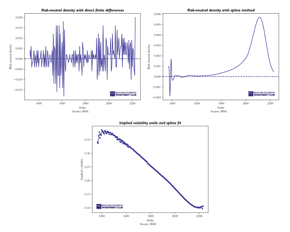
First attempt: direct finite differences

We select the largest consecutive block of strikes spaced exactly $\Delta K = 5$ points apart, yielding 183 observations, and apply the formula directly to market mid-prices. The resulting density, however, is erratic and takes on negative values for roughly half the strike range, which is a clear sign that raw prices, affected by bid-ask bounce and discrete quoting, are too noisy to survive two rounds of numerical differentiation. Only about 52% of the estimated density values are positive, confirming that this naive approach is not viable in practice.

Smoothing via implied volatility splines

A standard remedy proposed by Shimko (1993) [2] is to work in implied-volatility space rather than directly in price space. The idea is as follows: instead of differentiating noisy market prices, we first fit a smooth curve to the observed implied volatility smile, and then translate it back into call prices through the Black–Scholes formula before applying Breeden–Litzenberger.

Concretely, we fit a cubic smoothing spline to the implied volatility as a function of strike. Rather than forcing the curve to pass exactly through every data point, which would overfit to market microstructure noise, the smoothing parameter allows a small controlled amount of residual error in exchange for a smoother fit. We then evaluate the spline on a fine grid of 400 equally-spaced points spanning the observed strike range, and reprice each point using the Black–Scholes formula with the fitted implied volatility. The resulting call price curve is smooth by construction, and its second derivative, scaled by $e^{rT}$ , gives the risk-neutral density.

The improvement is striking: the smoothed density is everywhere non-negative, unimodal, and integrates to approximately 0.99 over the observed strike range (the small shortfall from 1 reflects the finite support of the grid, not a normalisation failure). The implied mean of the distribution is close to the forward price providing a reassuring sanity check on the procedure.

We present the graphs for the reconstruction of the risk-neutral density with the 2 approaches and the spline fit. Figure 2 illustrates that the spline method is not without its own limitations. In the far left tail, the density exhibits a sharp spike followed by negative values. This breakdown is a known limitation of spline-based smoothing: in regions where observed strikes are sparse or where the implied volatility smile changes curvature rapidly, the spline can oscillate and produce implausible density estimates. Nevertheless, the central body of the distribution, which concentrates the vast majority of the probability mass, remains well-behaved and is what we rely on for the time series analysis that follows.

Having validated the procedure on a single surface, we extend it systematically across the full dataset, which spans 2,681 trading days from January 2015 to August 2025. For each date, we select the expiry closest to 30 calendar days ahead, as it ensures a consistent horizon across time while keeping the density well-identified by a sufficient number of liquid strikes. We then apply the spline-based Breeden–Litzenberger procedure described above and record the full density $q(K;\,t)$ for each date $t$ . Consequently, we computed the 4 standardized moments of the distribution over time: mean, variance, skewness and kurtosis.

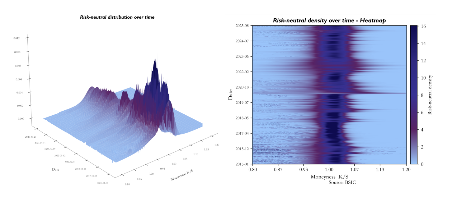The figures present the risk-neutral density extracted daily from SPX options between January 2015 and August 2025, displayed as both a three-dimensional surface and a heatmap. The heatmap encodes time on the vertical axis, with January 2015 at the bottom and August 2025 at the top, and moneyness on the horizontal axis, where darker navy corresponds to low density mass and the bright band marks where the market concentrates probability.

The dominant feature of both representations is the persistent concentration of density just above $K/S = 1.00$ , confirming that the at-the-money region consistently carries the highest probability mass across the entire sample. The slight rightward shift of the peak, sitting closer to $1.02$ – $1.03$ rather than exactly at $1.00$ , is consistent with the positive risk-neutral drift priced into the index.

The horizontal variation in the heatmap is equally informative. The bright band narrows and intensifies during calm periods, most visibly throughout 2017–2019, signalling that the market was pricing outcomes with high conviction around the current spot level. Conversely, the band widens and the surrounding density brightens during stress episodes. The 2020 COVID shock stands out as the clearest example, with a notably diffuse and elevated density spreading across a broad range of moneyness values.

Finally, the persistent asymmetry between the put side ( $K/S < 1.00$ ) and the call side reflects the structural negative skew of the risk-neutral distribution, a well-documented consequence of crash aversion and the equity risk premium embedded in SPX options throughout the sample.

From Risk-Neutral Densities to Implied Volatility

Once the risk-neutral density has been recovered, the natural next step is to summarize it through its moments and show how these moments connect to the volatility measures used in practice. This is the crucial bridge between the first part of the article, which extracts the full distribution from option prices, and the second part, which uses the risk-neutral distribution to reconstruct implied volatility, VIX, SVIX [3] within one coherent framework.

First, we show how to back-out Black-Scholes implied volatility from our estimate of the risk-neutral variance. Under Black-Scholes, the terminal price has the closed-form solution

$S_{T} = S_{0}\,e^{\left(r - \frac{1}{2}\sigma^{2}\right)T + \sigma W(T)}$

With $W(T) \sim \mathcal{N}(0,\,T)$ , which means that $S_{T}$ follows a lognormal distribution, which is handy since the moments of a lognormal distribution are known:

$\mathrm{Var}^{\mathbb{Q}}\!\left[S_{T}\right] = S_{0}^{2}\,e^{2rT}\!\left(e^{\sigma^{2}T}-1\right) = F^{2}\!\left(e^{\sigma^{2}T}-1\right)$

Let $\sigma_{\mathrm{RND}}^{2}$ denote our risk-neutral variance estimate we set $\mathrm{Var}^{\mathbb{Q}}\!\left[S_{T}\right] = \sigma_{\mathrm{RND}}^{2}$ and solve for $\sigma$ , the Black-Scholes implied volatility, which is consistent with the VIX index time series.

$\sigma_{\mathrm{implied}} = \sqrt{\frac{1}{T}\ln\!\left(1 + \frac{\sigma_{\mathrm{RND}}^{2}}{S^{2}e^{2rT}}\right)} = \sqrt{\frac{1}{T}\ln\!\left(1 + \frac{\sigma_{\mathrm{RND}}^{2}}{F^{2}}\right)}$

This expression simply states that implied volatility can be derived from the risk-neutral variance extracted from the density. In other words, once the distribution has been estimated, volatility is no longer an external input: it is a moment of that same distribution. This observation will be central below, because both VIX and SVIX can be interpreted as particular transformations of the same option-implied risk-neutral variance information.

From Implied Variance to VIX, SVIX, and Martin’s Bound

The result at the centre of this section is due to Ian Martin [3], who derives a lower bound on the equity risk premium using only the prices of index options. Working in a general, arbitrage-free framework, Martin shows that the expected excess return on the market under the historical probability $\mathbb{P}$ equals the risk-neutral variance of the market return minus a covariance term that depends on the joint behaviour of the stochastic discount factor and realized returns. Under a minimal sign restriction on the stochastic discount factor, the Negative Correlation Condition (NCC), which holds in virtually all standard macro-finance models, this covariance term is non-positive, and risk-neutral variance becomes a lower bound on the equity premium. Martin constructs the SVIX index as the square root of annualized risk-neutral variance and shows that, over his 1996–2012 sample, the bound appears approximately tight: the average level of SVIX² matches conventional estimates of the equity premium, and predictive regressions fail to reject the hypothesis that SVIX² equals the equity premium. The result is notable: option-implied variance directly bounds expected returns, without any model assumptions. The logic is powerful because it links an observable quantity from option prices to an object, expected returns under the historical probability $\mathbb{P}$ , that is usually much harder to measure directly.

Our contribution is to carry this logic into the 2015–2025 sample, after first building the risk-neutral density day by day from SPX options. The advantage of proceeding in this order is that the empirical quantities used in the second half of the paper are now tightly connected to the first: the density yields the variance, the variance yields implied volatility, and implied volatility leads naturally to VIX, SVIX, and Martin’s lower bound.

The exposition therefore proceeds in three steps. First, we recall the stochastic-discount-factor decomposition that underlies Martin’s result. Second, we relate VIX and SVIX to the variance extracted from the estimated density, clarifying why in our implementation VIX can be approximated directly from this. Third, we compare Martin’s original evidence with our more recent decade and discuss the implications for predictability.

Martin’s Lower Bound and the Stochastic Discount Factor

The starting point is the standard stochastic discount factor (SDF) identity: the price of any payoff equals the expectation of that payoff multiplied by the SDF. Applied to the market portfolio, this identity delivers the decomposition that makes the link between expected returns under $\mathbb{P}$ and option-implied variance transparent. The SDF $M_{T}$ is chosen to make the pricing work under the historical probability $\mathbb{P}$ :

$S = E^{\mathbb{P}}\!\left[M_{T}\, S_{T}\right] = \frac{1}{R_{f}}\,E^{\mathbb{Q}}\!\left[S_{T}\right]$

Dividing both sides by $S$ and defining the gross return $R_{T} = S_{T}/S$ :

$1 = E^{\mathbb{P}}\!\left[M_{T}\,R_{T}\right]$

We now decompose this expectation using the identity $E[XY] = E[X]\,E[Y] + \mathrm{Cov}(X,Y)$ :

$1 = E^{\mathbb{P}}\!\left[M_{T}\right] E^{\mathbb{P}}\!\left[R_{T}\right] + \mathrm{Cov}^{\mathbb{P}}\!\left(M_{T},\,R_{T}\right)$

To pin down $E^{\mathbb{P}}\!\left[M_{T}\right]$ , apply the same SDF identity to the risk-free asset, which pays $R_{f}$ with certainty:

$E^{\mathbb{P}}\!\left[M_{T}\right] = \frac{1}{R_{f}}$

Substituting back and rearranging, the expected return on the market satisfies:

$1 = \frac{1}{R_{f}}\,E^{\mathbb{P}}\!\left[R_{T}\right] + \mathrm{Cov}^{\mathbb{P}}\!\left(M_{T},\,R_{T}\right)$

The covariance term is unobservable under $\mathbb{P}$ , so we bridge to the risk-neutral measure $\mathbb{Q}$ , where option prices live. Using the change of measure $E^{\mathbb{Q}}[\,\cdot\,] = R_{f}\,E^{\mathbb{P}}\!\left[M_{T}\cdot\right]$ and the fact that $E^{\mathbb{Q}}\!\left[R_{T}\right] = R_{f}$ by no-arbitrage, one can show:

$\mathrm{Var}^{\mathbb{Q}}\!\left(R_{T}\right) = R_{f}\!\left(E^{\mathbb{P}}\!\left[R_{T}\right] - R_{f}\right) - R_{f}^{2}\,\mathrm{Cov}^{\mathbb{P}}\!\left(M_{T},\,R_{T}\right)$

Rearranging the pricing identity yields a decomposition of the expected excess return into an observable risk-neutral-variance component and a covariance term that captures how payoffs comove with marginal utility.

$E^{\mathbb{P}}\!\left[R_{T}\right] - R_{f} = \frac{1}{R_{f}}\,\mathrm{Var}^{\mathbb{Q}}\!\left(R_{T}\right) - \mathrm{Cov}^{\mathbb{P}}\!\left(M_{T},\,R_{T}\right)$

The first term on the right-hand side is attractive because it is observable from option prices: it is the risk-neutral variance of the market return. The second term is more subtle. It depends on the joint behaviour of the stochastic discount factor and realized returns under the historical probability measure, and for this reason it cannot be backed out from option prices alone.

This distinction is essential for the interpretation of Martin’s result. Options pin down the risk-neutral distribution, hence its variance, skewness and kurtosis; they do not directly reveal the historical distribution, nor the covariance between returns and the SDF. Any lower-bound argument must therefore control this covariance term separately.

Economically, the covariance term is large when bad market outcomes coincide with states in which marginal utility is high. In recession or disaster states, investors value wealth more, the SDF rises, and equities tend to perform poorly; this makes the covariance negative and increases the required equity premium above the pure variance component. The stochastic discount factor satisfies $M_{T} \propto u^{\prime}\!\left(W_{T}\right)$ , which is decreasing and convex in wealth for any risk-averse investor. In normal times, wealth fluctuations are small and marginal utility is nearly flat across states, so the comovement between $M_{T}$ and $R_{T}$ is moderate. In a crisis, equity losses push investors into the steep region of $u^{\prime}(W)$ where each additional dollar of loss produces a disproportionately large spike in marginal utility, and this spike occurs precisely in the states where returns are most negative. The convexity of marginal utility therefore acts as an amplifier: the deeper the drawdown, the more $M_{T}$ and $R_{T}$ move in opposite directions, and the more negative their covariance becomes.

Martin’s key assumption is a weak sign restriction ensuring that this covariance cannot overturn the variance term. Under his condition, risk-neutral variance becomes a lower bound on the expected excess return on the market. More precisely, under the Negative Correlation Condition (NCC) one has:

$\mathrm{Cov}^{\mathbb{P}}\!\left(M_{T},\,R_{T}\right) \leq 0$

and therefore, the expected excess return satisfies:

$E^{\mathbb{P}}\!\left[R_{T}\right] - R_{f} \geq \frac{1}{R_{f}}\,\mathrm{Var}^{\mathbb{Q}}\!\left(R_{T}\right)$

The importance of the inequality is immediate: once the covariance term is known to be non-positive, an object measured directly from options becomes informative about the minimum compensation investors require to hold the market. This is the theoretical channel through which SVIX enters the equity-premium discussion.

VIX and SVIX relationship

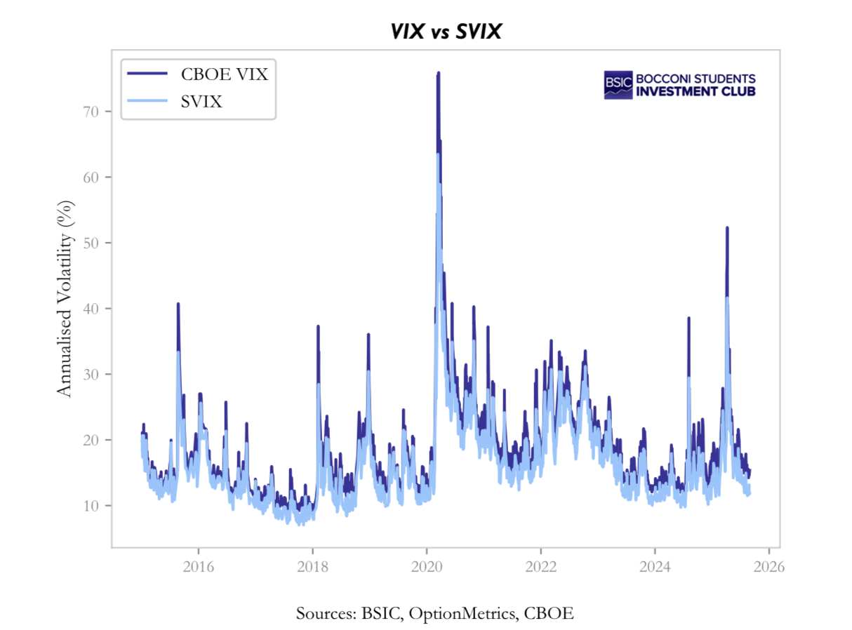
Both VIX and SVIX are built from option prices, but they encode different aspects of the risk-neutral distribution. VIX is the standard market volatility index and places relatively more weight on far out-of-the-money options, especially puts. SVIX, instead, is the variance object that appears naturally in Martin’s decomposition and is more directly connected to the lower bound on expected returns.

The CBOE VIX is defined from a continuum of out-of-the-money puts and calls as

$\mathrm{VIX}^{2} = \frac{2e^{rT}}{T}\!\left[\int_{0}^{F}\frac{P(K)}{K^{2}}\,dK + \int_{F}^{\infty}\frac{C(K)}{K^{2}}\,dK\right]$

The 1/K² weighting is what makes VIX especially sensitive to the left tail of the distribution. Deep out-of-the-money puts receive a large weight, so VIX rises not only when overall variance increases, but also when crash insurance becomes particularly expensive.

SVIX is defined more directly as the annualized risk-neutral variance of the market return. In Martin’s notation it can be written as

$\mathrm{SVIX}^{2} = \frac{2e^{rT}}{T S^{2}}\!\left[\int_{0}^{F} P(K)\,dK + \int_{F}^{\infty} C(K)\,dK\right]$

or, equivalently (see appendix for detailed derivation):

$\mathrm{SVIX}^{2} = \frac{1}{T}\,\mathrm{Var}^{\mathbb{Q}}\!\left(R_{T}\right)$

The comparison is informative. Because VIX emphasizes tail insurance more than SVIX, one typically has VIX greater than or equal to SVIX. The two indices coincide only in limiting cases in which higher-moment asymmetries are negligible; in actual equity-index data, the gap between them is persistent precisely because downside tail risk is persistently priced.

This difference matters for interpretation. The spread VIX² minus SVIX² measures the portion of implied volatility associated with asymmetry and tail thickness, while the ratio SVIX/VIX indicates how much of total implied volatility reflects broad variance rather than tail-specific fear. In stress episodes the spread widens and the ratio falls; in calm periods the opposite tends to happen.

In our implementation, however, we do not need to recover VIX by numerically evaluating the option integral every time. Once the risk-neutral density has been estimated, the relevant second moment is already available. Since the first part of the paper delivers a smooth estimate of the density, we can compute the implied variance directly from that density and then map it into both the VIX and SVIX objects. Concretely, with forward price F, we compute:

$\mathrm{SVIX}^{2} = \frac{\mathrm{Var}^{\mathbb{Q}}\!\left(R_{T}\right)}{T} = \frac{\sigma_{\mathrm{RND}}^{2}}{T S^{2}}$

This approximation is legitimate because the option integral and the second moment of the risk-neutral density are two representations of the same object. Breeden–Litzenberger tells us that option prices encode the density; integrating option prices across strikes recovers the second moment, while integrating the estimated density against the relevant payoff does the same in a more direct and numerically stable way.

$\int_{0}^{F} P(K)\,dK + \int_{F}^{\infty} C(K)\,dK = \frac{\sigma_{\mathrm{RND}}^{2}}{2e^{rT}}$

For this reason, once the density has been smoothed and its moments have been estimated, using this variance measure is a practical shortcut rather than a conceptual simplification. It avoids re-integrating noisy and discretely quoted option prices, while remaining anchored to the same no-arbitrage quantity. This is why, in our empirical exercise, VIX can be approximated directly from this measure without loss of economic meaning. In practice, for the strategy analysis and the regression tests, we use the SVIX computed from the risk-neutral density as the core signal, while the official CBOE VIX (at daily frequency) serves as an external benchmark to verify consistency.

The VIX-SVIX Spread and Higher Moments

The gap between VIX² and SVIX² is especially useful because it summarizes the role of higher moments in option prices. Since both measures share the same variance backbone, their difference isolates the component of implied volatility generated by skewness and kurtosis rather than by dispersion alone.

Let $x$ denote the centered normalized log return under the risk-neutral measure and let $\mu_{k}$ be its cumulants. A Taylor expansion around the second moment gives:

$\mathrm{VIX}^{2}\,T \approx E^{\mathbb{Q}}\!\left[x^{2}\right] - \frac{2}{3}\,E^{\mathbb{Q}}\!\left[x^{3}\right] + \frac{1}{2}\,E^{\mathbb{Q}}\!\left[x^{4}\right] + o\!\left(x^{5}\right)$

$\mathrm{SVIX}^{2}\,T \approx E^{\mathbb{Q}}\!\left[x^{2}\right] = \mathrm{Var}^{\mathbb{Q}}[x]$

We can rewrite the expansion in terms of standardized risk neutral skewness ( $\gamma$ ) and excess kurtosis ( $\kappa$ ). Here $\sigma_{R}$ represents the risk-neutral volatility of the log-returns.

$\mathrm{VIX}^{2} - \mathrm{SVIX}^{2} \approx -\frac{2}{3}\,\gamma\,\sigma_{R}^{3} + \frac{1}{2}\,\kappa\,\sigma_{R}^{4}$

In our data, risk-neutral skewness is persistently negative, exactly as one would expect for an equity index with pronounced crash aversion. Excess kurtosis is also positive. Both features push VIX² above SVIX², so the spread becomes a compact summary of how much the left tail and fat tails matter for option prices at each point in time.

Testing Martin’s Evidence in our sample

A natural question is whether Martin’s original evidence survives in the more recent decade. In his 1996–2012 sample, the lower bound appeared approximately tight: regressing realized excess returns on SVIX² produced a slope close to one, suggesting that the covariance term omitted by the bound was often small in practice.

$E^{\mathbb{P}}\!\left[R_{T}\right] - R_{f} = \alpha + \beta\,\mathrm{SVIX}^{2} + \varepsilon$

That result was important because it implied that, at least on average, option-implied variance tracked a large share of the equity premium. In other words, the variance-only component was not merely a lower bound in theory; empirically, it seemed close to the full object of interest.

When we repeat the exercise over 2015–2025, the picture changes materially. Using non-overlapping monthly observations, our estimates imply a much larger coefficient: $\beta \approx 5.2$ . The lower bound still holds directionally, but it is far from tight.

The statistical evidence confirms the break with Martin’s original sample. The null that the intercept is zero and the slope is one is decisively rejected, and the result is robust to bootstrap confidence intervals and sub-sample checks. The interpretation is straightforward: in the last decade, the covariance term left outside the lower bound has become economically important.

This is consistent with the macro character of the period. COVID, the inflation shock, rapid rate normalization and repeated regime uncertainty increased the extent to which bad equity outcomes coincided with high-marginal-utility states. As a result, the variance component remained informative, but a much larger share of the equity premium was generated by time-varying “crash covariance” rather than by variance alone.

SVIX, VIX and linear spread predictive power

We now ask whether VIX² and the spread VIX²−SVIX² carry predictive power beyond what SVIX² alone provides. Since the spread isolates the higher-moment component of option-implied variance, namely skewness and kurtosis rather than dispersion, it is the natural candidate for testing whether the tail-risk premium constitutes a distinct forecasting channel.

Univariate regressions reveal that all three signals, $\mathrm{SVIX}^{2}$ , $\mathrm{VIX}^{2}$ and the spread, are individually highly significant predictors of subsequent excess returns, with $R^{2}$ values of 0.061, 0.066, and 0.065 respectively. The near-equality of these figures is the central finding: it implies that there is a single latent factor, which we may call “option-implied risk perception”, that all three indicators capture in slightly different proportions but with equivalent overall power. The slope coefficients differ, with $\widehat{\beta} \approx 5.2$ for $\mathrm{SVIX}^{2}$ , $\widehat{\beta} \approx 3.6$ for $\mathrm{VIX}^{2}$ , and $\widehat{\beta} \approx 9.2$ for the spread, but these differences are mechanical consequences of scaling (considering the almost perfect correlation): smaller regressors receive proportionally steeper slopes to explain the same variation in the dependent variable, and $R^{2}$ is the scale-free measure that reveals the underlying equivalence.

To test for distinct channels more directly, we estimate the decomposed regression

$y_{t} = \alpha + \beta_{1}\,\mathrm{SVIX}_{t}^{2} + \beta_{2}\!\left(\mathrm{VIX}_{t}^{2} - \mathrm{SVIX}_{t}^{2}\right) + \varepsilon_{t}$

where $\beta_{1}$ captures the pure variance channel and $\beta_{2}$ captures the tail-premium channel. The results are $\widehat{\beta}_{1} = 2.07$ ( $p = 0.44$ ) and $\widehat{\beta}_{2} = 6.19$ ( $p = 0.08$ ), with a combined $R^{2} = 0.067$ that barely exceeds the univariate values. Neither coefficient is significant at the 5% level. The multicollinearity between the two regressors, which arises because variance and tail premium move together as risk-neutral skew becomes more negative when volatility rises, prevents OLS from stably attributing the common predictive content to one channel or the other.

These results have a clear interpretation within Martin’s framework. The theoretical decomposition of VIX into a variance component (SVIX) and a higher-moment component (the spread) is confirmed in the data: the spread is strictly positive, averages 27% of $\mathrm{VIX}^{2}$ , and widens in stress episodes exactly as theory predicts. But this structural decomposition does not map into separable predictive channels. In the option market, variance, skewness, and kurtosis are driven by a common underlying factor, the intensity of risk aversion, and they move in lockstep.

A complementary result

The regressions and the decomposition establish that option-implied variance is a statistically significant predictor of excess returns and that $\mathrm{SVIX}^{2}$ , $\mathrm{VIX}^{2}$ , and the spread capture a single common factor with equivalent explanatory power. A natural follow-up question is whether this predictive content can be translated into economic value by an investor who acts on the signal in real time. To answer this, we construct a very simple equity-timing strategy and compare its risk-adjusted performance against a passive Buy&Hold benchmark. The allocation rule scales equity exposure to the S&P 500 according to the current level of each signal relative to its own history:

$\alpha_{t} = \min\!\left(2,\;\max\!\left(0,\;\frac{X_{t}^{2}}{\bar{X}_{t-1}^{2}}\right)\right)$

where $X_{t}^{2}$ is either $\mathrm{SVIX}^{2}$ , $\mathrm{VIX}^{2}$ , or spread observed on date $t$ , and $\bar{X}_{t-1}^{2}$ is its expanding historical mean computed using only information available up to the previous month. The remaining is invested at the risk-free rate. The allocation is bounded between zero and two to prevent extreme leverage. Rebalancing occurs on non-overlapping monthly cycles aligned to option expiry dates.

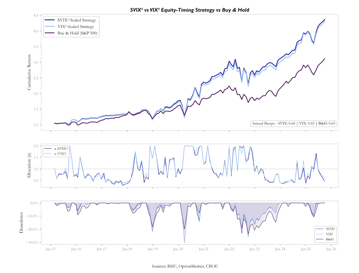
The three timing strategies produce annualised returns all above the 11.5% delivered by Buy & Hold. However, the additional return comes entirely from increased risk exposure: the strategies have annualised volatilities and maximum drawdowns substantially higher than the passive benchmark. On a risk-adjusted basis, none of the three strategies outperforms the market: the annualised Sharpe ratios are 0.60, 0.59, and 0.55, all below the benchmark’s 0.65.

This outcome is not a contradiction of the predictive regressions, but rather their necessary complement. The regressions measure the average linear relationship between the signal and subsequent returns across the full sample, whereas the strategy is a sequential, real-time implementation in which early estimates of the expanding mean are based on few observations.

The near-equivalence of the three strategies confirms, on an independent methodological footing, the conclusion reached through the regressions: the three signals are functionally interchangeable because they reflect a single underlying factor, and neither the pure variance channel nor the tail-premium channel offers a separable edge. The spread-based strategy performs marginally worse (Sharpe 0.55), consistent with the fact that the spread, while carrying the same $R^{2}$ as the other two signals in the univariate regression, has a lower correlation with SVIX and VIX allocations and tends to diverge from the variance-based signals precisely in the episodes where variance turns out to be the more reliable guide.

Conclusion

This article has followed a single analytical thread from raw option prices to a complete characterisation of what the equity option market knows, and does not know, about future returns.

The starting point was the Breeden–Litzenberger identity, implemented on S&P 500 option data spanning 2015 to 2025. We showed that a spline-based smoothing procedure in implied-volatility space produces a risk-neutral density that is non-negative and unimodal, providing a day-by-day reconstruction of how the market prices variance, skewness, and tail risk over an entire decade.

From the extracted densities we computed SVIX, the annualised risk-neutral standard deviation that enters Martin’s (2017) lower bound on the equity premium, together with VIX and the linear spread, which isolates the higher-moment component of option-implied variance. The three objects behave as theory predicts: VIX exceeds SVIX on every day in the sample, the spread averages 27% of $\mathrm{VIX}^{2}$ , and both the spread and the level of implied variance widen sharply during stress episodes.

The central empirical finding is twofold. First, Martin’s lower bound holds but is far from tight: the Wald test rejects the null $\alpha = 0$ , $\beta = 1$ at the 1% level for both $\mathrm{SVIX}^{2}$ and $\mathrm{VIX}^{2}$ , with slope estimates approximately five times the theoretical prediction. This implies that the covariance between returns and the stochastic discount factor has become the dominant component of the equity premium. The result is consistent with the macroeconomic character of the 2015–2025 decade: a global pandemic, the sharpest inflation and rate cycle in forty years, and recurring events of acute market stress all increased the extent to which adverse equity outcomes coincided with states of high marginal utility, inflating the “crash-covariance” channel well beyond the levels observed in Martin’s original sample.

Second, the predictive content of option-implied variance is real, but the same across indexes. $\mathrm{SVIX}^{2}$ , $\mathrm{VIX}^{2}$ , and the spread all predict excess returns with similar $R^{2}$ values and the decomposed regression cannot reject the hypothesis that both channels are driven by a single common factor. The theoretical decomposition of VIX into a variance component and a tail-risk component is confirmed structurally in the data, but it does not map into separable predictive channels: variance, skewness, and kurtosis move together, propelled by a single underlying factor that we may interpret as the market’s aggregate intensity of risk aversion.

Finally, the equity-timing strategies we construct to translate the statistical signal into economic performance confirm both conclusions. This complementary result should be interpreted with care. It does not imply that option-implied variance is uninformative, nor that the equity premium is unforecastable. It means that a simple, single-signal timing rule applied at monthly frequency is not sufficient to convert the information embedded in the risk-neutral density into risk-adjusted alpha. More sophisticated implementations may indeed reach a different conclusion and represent a natural direction for future work.

Appendix: The two representations for the SVIX index

Let $R_{T} = S_{T}/S_{t}$ be the gross linear return between two dates. By definition, the SVIX index over this period is the annualized risk-neutral variance of this simple return under $\mathbb{Q}$ . Let’s implement this definition:

$\mathrm{Var}_{t}^{\mathbb{Q}}\!\left(R_{T}\right) = \frac{1}{S_{t}^{2}}\,\mathrm{Var}_{t}^{\mathbb{Q}}\!\left(S_{T}\right) = \frac{1}{S_{t}^{2}}\!\left(E_{t}^{\mathbb{Q}}\!\left[S_{T}^{2}\right] - \left(E_{t}^{\mathbb{Q}}\!\left[S_{T}\right]\right)^{2}\right)$

Now, the expected value under $\mathbb{Q}$ coincides with the forward price $F_{t,T}$ . The key manipulation concerns the second moment, which can be expressed in an option-representation, by simply exploiting the following identity (the proof can be tackled by removing the expected value operator and check for a generic $(x - K)^{+}$ under the integral sign).

$\frac{1}{B_{t}(T)}\,E_{t}^{\mathbb{Q}}\!\left[S_{T}^{2}\right] = 2\int_{0}^{\infty} C_{t}(K,T)\,dK$

From here we further split the integral at $F_{t,T}$ and using the put-call parity to re-write in-the-money calls as out-of-the-money put options (of course the lower bound of the integration interval cannot be negative):

$\mathrm{Var}_{t}^{\mathbb{Q}}\!\left(R_{T}\right) = \frac{2\,B_{t}(T)}{S_{t}^{2}}\!\left[\int_{0}^{F_{t,T}} P_{t}(K,T)\,dK + \int_{F_{t,T}}^{\infty} C_{t}(K,T)\,dK\right]$

Which is exactly the expression mentioned multiple times throughout the article.

References

Breeden, Douglas T.; Litzenberger, Robert H. (1978), Prices of State-Contingent Claims Implicit in Option Prices,, Journal of Business.
Shimko, David C. (1993), Bounds of Probability, Risk.
Martin, Ian W. (2017), What Is the Expected Return on the Market?, Quarterly Journal of Economics.
CBOE (2019), “VIX White Paper”, Chicago Board Options Exchange.

Published by BSIC on 29 March 202629 March 2026

0 Comments

Leave a Reply Cancel reply

Understanding Convexity Bias in STIR Futures Markets

Market Recap 29/03/2026

Market Recap 08/03/2026