The SABR model is like the Vega/Vanna Volga Approach, in that it is a method of interpolating the implied volatility surface. Given the dynamics of the forward rate, the stochastic instantaneous volatility, and the Black model, we get an algebraic expression that the Black Implied Volatility must satisfy.
Given traded and liquid options, we fit the SABR model on the observed smile and estimate the parameters. Using these parameters, we can estimate Black Implied Vol to price exotics and vanilla swaptions at various points on the vol grid. The underlying assumption is: let the market tell us what to do. We take the opinion of the market on liquid points on the vol grid to estimate parameters and extrapolate/interpolate them to other illiquid/non-traded points in order to price options.
The SABR model
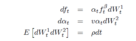
The SABR model assumes that the forward rate and the instantaneous volatility are driven by two correlated Brownian motions:
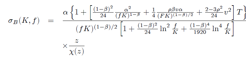
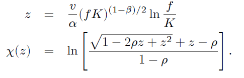
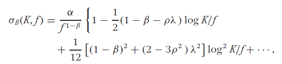
The expression that the implied volatility must satisfy is 1
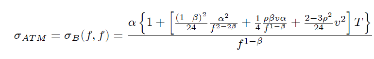
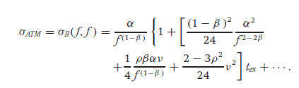
When  (for ATM options), the above formula for implied volatility simplifies to:
where
- α is the instantaneous vol;
- ν is the vol of vol;
- ρ is the correlation between the Brownian motions driving the forward rate and the instantaneous vol;
- β is the CEV component for forward rate (determines shape of forward rates, leverage effect and backbone of ATM vol).
The local volatility function, which includes the stochastic instantaneous vol and the deterministic function of F, expressed as % of forward rate is given by:

β is one of the key parameters and affect many fundamental characteristics of the model. β is the exponent for the forward rate or the CEV exponent and effects the distribution
- β = 1 – stochastic lognormal rates
- β = 0 – stochastic normal rates
- β = ½ – stochastic CIR model (with 0 drift)
As the CEV component, β helps capture leverage effect without changing the underlying instantaneous vol (α). So, if 0<β<1 (as in SABR), we have leverage effect –volatility falls as F increases.
The dynamics of the Implied Volatility formula
For strikes not too far from the forward rate, the Implied Volatility formula can be approximated as
where λ measures the strength of vol-of-vol against the local volatility at the current forward rate

The dynamics of  can be broken down into 3 parts – backbone, smile(convexity) and skew.
1- The backbone
The backbone  is the change in ATM vol for a change in the forward rate. The backbone is almost entirely determined by the exponent β: with β = 0 (a stochastic vol Gaussian model) we get a steeply downward sloping backbone, and with β = 1 (a stochastic vol lognormal model) we get a nearly flat backbone – as in the Black and Scholes model. To plot the backbone for given values of α, β, ρ and ν, we change the value of f and compute the ATM vol assuming that K=f (ie, using the ATM vol formula).
2- The skew
The skew is given by  and is the sum of two components:
- the Beta Skew
 , which makes the implied vol downward sloping in terms of K (because 0<=beta<=1). It arises because of the leverage effect built into the local volatility (assuming constant instantaneous vol) – ie, because the local volatility
  is a decreasing function of the forward price;
 - the Vanna Skew
 , which is caused by the correlation between instantaneous volatility and f. Typically, the volatility and asset price are negatively correlated, so on average, the volatility α would decrease (increase) when the forward f increases (decreases). It thus seems unsurprising that a negative correlation ρ causes a downward sloping vanna skew (lower vol at higher strikes).
Interestingly, the slope of the backbone will be twice as steep as the slope of the smile due to the β-component of the skew. Basically, according to the backbone, the ATM vol falls as f increases. The skew is also affected by the backbone multiplier – so as the f increases, the beta component of skew makes the implied vol at a K rise, but ATM vol falls due to backbone: thus the impact on skew is dampened.
3- The convexity
The convexity term responsible for the smile is
![]()
and can also be decomposed into two terms:
- the smile induced by the Skew effect
 . It is essentially a second order effect of the skew term for bigger moves from
  ;
;
- the smile induced by the Volga effect

![]()
Intuitively, the smile arises because unusually large movements of the forward f happen more often when the volatility α increases, and less often when α decreases, so strikes K far from f represent on average, high volatility environments.
How to fit the Market Data
1- Beta
β has little effect on the shape of the surface/smile (as a snapshot at a given f and time to expiry), but:
- β is the primary determinant of backbone – so it determines how the surface shifts up and down as f moves;
- it massively effects the greeks – especially the delta – so we use an adjusted delta with SABR – Bartlett’s delta – to reduce the sensitivity of delta to the choice of β (more on this later).
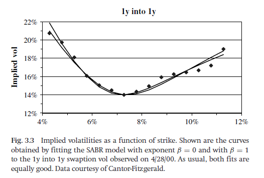
To elaborate on the first point above, market smiles can be fit equally well with any specific value of β. Because The exponent β and correlation ρ affect the volatility smile in similar ways – (they both cause a downward sloping skew in  as the strike K varies), from a single market snapshot of as a function of K at a given f, it is difficult to distinguish between the two parameters.
For instance, in the figure below we fit the SABR parameters α, ρ, ν with β = 0 and, then, re-fit the parameters α, ρ, ν with β = 1. Note that there is no substantial difference in the quality of the fits, despite the presence of market noise.
Because β has little effect on the shape of the surface, beta is usually set using a regression or according to our belief of the distribution of rates, and then we estimate the other parameters. Hence, we generally don’t fit smiles to estimate beta. β can be determined from:
- historical observations of the backbone. Taking the log of the main SABR ATM vol formula, we get
 As the terms after log(f) are very small and can be ignored, we estimate β regressing the log of historical ATM vol to the log of forward rate. The issue with this regression is that both alpha and f are stochastic, hence there is a lot of noise;
 - “aesthetic considerations”, based on our belief of the distribution of f:
- β = 1 (stochastic lognormal) – proponents say log normal models are “more natural” or believe that the horizontal backbone best represents their market. These proponents often include desks trading foreign exchange options;
- β = 0 (stochastic normal, with negative rates) – Proponents usually believe that a normal model, with its symmetric break-even points, is a more effective tool for managing risks, and would claim that β = 0 is essential for trading markets like Yen interest rates, where the forwards f can be negative or near zero;
- β = 1/2 (stochastic CIR) models – usually US interest rate desks that have developed trust in CIR models.
2- Other parameters
With β given, fitting the SABR model is a straightforward procedure. The three parameters α, ρ, and ν have different effects on the curve:
- α controls the overall height of the curve;
- ρ controls the curve’s skew;
- ν controls how much smile the curve exhibits.
Because of the widely separated roles these parameters play, the fitted parameter values tend to be very stable, even in the presence of large amounts of market noise. It is usually more convenient to use the at-the-money volatility σATM , β, ρ, and ν as the SABR parameters instead of the original parameters α, β, ρ, ν. In the generic volatility formula of SABR we express all the α terms as a function of σATM (basically we manipulate the equation such that α is removed). The parameter α is then found whenever needed by inverting the main ATM Implied Vol formula on the fly (given below). This inversion is numerically easy since the higher order terms are small.
 With this parameterization, fitting the SABR model requires fitting ρ and ν to the implied volatility curve, with σATM and β given. In many markets, the ATM volatilities need to be updated frequently, say once or twice a day, while the smiles and skews need to be updated infrequently, say once or twice a month. With the new parameterization, σATM can be updated as often as needed, with ρ, ν (and β) updated only as needed.
Some observation from fitting SABR on US swaptions and rates options market
The smile and skew depend heavily on the time-to exercise. Smile dominates in shorter maturities, as the vol of vol ν is very high for short dated options, and decreases as the time-to-exercise increases. This matches general experience: in most markets there is a strong smile for short-dated options which relaxes as the time-to-expiry increases; consequently the volatility of volatility ν is large for short dated options and smaller for long-dated options, regardless of the particular underlying.
Experience with correlations is less clear: in some markets a nearly flat skew for short maturity options develops into a strongly downward sloping skew for longer maturities. In other markets there is a strong downward skew for all option maturities, and in still other markets the skew is close to zero for all maturities.
For swaption, there is little dependence of the market skew and smile on the length of the underlying swap: both ν and ρ are fairly constant across tails.
The predicted dynamics of the smile matches market experience – whenever the forward price f changes, the implied volatility curve shifts in the same direction and by the same amount as the price f – this overcomes a massive problem with local vol models where the smile shifts in the opposite direction as f.
If β < 1, the “backbone” is downward sloping, so the shift in the implied volatility curve is not purely horizontal – the curve shifts up and down as the at-the-money point traverses the backbone.
Managing Smile Risk and the modified greeks
A big advantage of risk management with SABR is that greeks are consistent across any one smile (at a given maturity) and can be added. Since the SABR model is a single self-consistent model for all strikes K, the risks calculated at one strike are consistent with the risks calculated at other strikes. Therefore, the risks of all the options on the same asset and with the same maturity can be added together, and only the residual risk needs to be hedged. On the other hand, in the Black formula each strike has a different constant volatility, which essentially means we are using a different model at each K, which makes the risks not directly comparable across strikes.
According to the SABR model, the value of a call is  where the volatility
  is the SABR implied volatility. In other words, we can find the value of the option by plugging in the SABR implied volatility in the Black formula. However, due to the new stochastic volatility dynamics incorporated into the SABR implied volatility, a few changes need to be made to the option greeks. These changes are illustrated below.
Delta
1- Delta in original SABR
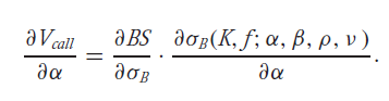
If we use the parameterization α, β, ρ, ν, so that , 
The first term is the regular Black delta.
The second term is the SABR model’s correction to the risk – Black vega*times the predicted change in the implied volatility σB caused by the change in the forward f. This change consists of –
- The option moving and down the smile – ie, caused by a sideways movement of the volatility curve in the same direction (and by the same amount) as the change in the forward price f.
- If β < 1 the volatility curve rises and falls as the at-the-money point traverses up and down the backbone.
Note – if we use the parameterization σAMT , β, ρ, and ν, delta is written as –
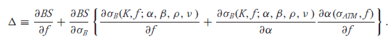
Where α is a function of σATM and f defined by the SABR ATM vol formula. The delta risk is now the risk to changes in f with σATM held fixed. The last term is just the change in α needed to keep σATM constant while f changes. Clearly this last term must just cancel out the vertical component of the backbone, leaving only the sideways movement of the implied volatility curve. Note that this term is zero for β = 1.
Theoretically, one should use the delta from the first parameterization to risk-manage books. In many markets, however, it may take several days for volatilities σB to change following significant changes in the forward price f. In these markets, using the second delta is a much more effective hedge.
For suppose one used from equation the first delta – when the volatility σATM did not immediately change following a change in f, one would be forced to re-mark α to compensate, and this re-marking would change the hedges. As σATM equilibrated over the next few days, one would mark α back to its original value, which would change the hedges back to their original value. This “hedging chatter” caused by market delays can prove to be costly.
Let us use the first delta formula for the rest of this section:
The adjustment term to Black Delta here only accounts for changes caused by the local vol function – that is, it accounts for systematic changes in implied vol as f changes (implicitly assuming that alpha remains constant). However, due to a non-zero correlation between alpha and f, the alpha changes too as f changes and hence the change in implied vol is both a function of implied volatility changing deterministically as f changes (as measured by local vol) as well the as the underlying stochastic vol (alpha) changing as f changes. This correction is made by Barlett.
2- Updated Bartlett Delta to account for changes in instantaneous vol caused by f
In the original SABR model, the delta hedge was calculated by shifting the current value of the underlying while keeping the current value of α fixed:
f → f + Δf, α → α.
However, since α and f are correlated, whenever f changes, on average α changes as well. A delta scenario which is more realistic than the above scenario is
f → f + Δf, α → α + δfα
The average change in α due to a change in the forward is given by
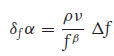
Hence, the new delta risk is given by

This incorporates the average change in instantaneous volatility caused by change in the underlying. The new term in the updated delta risk is just ρν/fβ times the classic SABR vega risk.
If the (classic SABR) vega risk and (classic SABR) delta risk are both hedged, then the Bartlett delta risk is also hedged. However, if we only hedge the classic SABR delta, this term new won’t be hedged.
An additional advantage of using the Bartlett adjusted delta is that it reduces the delta’s sensitivity to Beta (a problem we alluded to earlier). We noted earlier that Beta doesn’t effect the shape of the smile (and hence is difficult to estimate given a smile), however it effects the backbone and has a major impact on the delta.
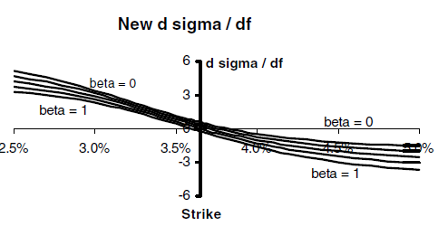
Remember that the original SABR delta only incorporated the volatility risk due to f changing through the local volatility – systematic change in the implied vol curve due to changes in the forward f expressed as ∂σ/∂f.
The figure below shows the ∂σ/∂f term from the original SABR article.

This term changes substantially with the value of beta, causing the Classic SABR delta’s sensitively to beta.
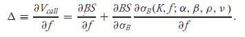
Now, the Bartlett adjusted delta accounts for the average change in α that occurs when f changes. Hence, the total volatility risk due to f changing is given by:
![]()
This term also makes the delta hedge relatively insensitive to the particular value of β chosen, especially
near the ATM point.
Why is the sensitivity to beta reducing with the updated delta? Adjusted delta hedges are not overly sensitive to which fraction of the skew/smile is arises from deterministic changes in the local volatility, and which arise from average changes in the local volatility in the adjusted delta (a division dictated to a large extent by beta)
Vega
1- Vega in Original SABR
Vega risk is the change in value when α changes by a unit amount
 Vega, in practice, can be found by bumping the instantaneous variance to α + δ, and then subtracting to determine the risk. It is traditional to scale vega so that it represents the change in value when the ATM volatility changes by a unit amount. Since δσATM = (∂σATM /∂α ) δα, the vega risk is
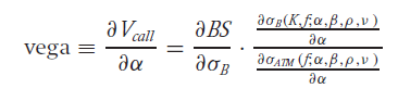
To leading order, ∂σB /∂α ≈ σB/α and ∂σATM /∂α ≈ σATM /α, so the vega risk is roughly given by
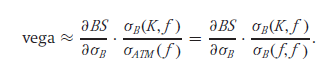 Hence, qualitatively, vega risks at different strikes are calculated by bumping the implied volatility at each strike K by an amount that is proportional to the implied volatility σB (K, f) at that strike. That is, in using the last equation above, we are essentially using proportional, and not parallel, shifts of the volatility curve to calculate the total vega risk of a book of options.
As in the case of delta, the original SABR vega above ignores that, in theory, due to the correlation between f and alpha, changes in the instantaneous vol should result in changes in f. We share the Bartlett adjusted vega bellow to account for this effect.
2- Updated Bartlett Vega to account for changes in instantaneous vol caused by f
As in the case of delta, the vega risk should be calculated from the scenario:
f → f + δαf, α → α + Δα
where δα f is the average change in f caused by the change in alpha. It can be shown that:
δαf = (ρfβ/ν) * Δα
Hence, the new vega risk is given by

where the first term is the classis SABR vega, and the second term captures how changes in f (induced by change in alpha) impacts the local vol. As in the case of the Bartlett Delta, an option that has the Classic SABR delta + vega hedged also has the Bartlett vega hedged (as it is hedged against changes in local vol).
Vanna and Volga
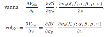 Since ρ and ν are determined by fitting the implied volatility curve observed in the marketplace, the SABR model has risks to ρ and ν changing. Vanna basically expresses the risk to the skew increasing, and volga expresses the risk to the smile becoming more pronounced. These risks are easily calculated by using finite differences on the formula for σB in the SABR equations, and can be hedged by buying and selling OTM options.
- See ‘Managing Smile Risk’ by Patrick S. Hagan, 2002, for derivation


2 Comments
Wdowiak · 20 December 2022 at 0:17
Thank you so much
Tanguy · 18 July 2024 at 16:51
Great explanation! Thanks