Introduction
The following article is heavily inspired by the paper “Investment Strategies with VIX and VSTOXX” (Stanescu, Tunaru, 2012) which analyzed different volatility trading strategies. The strategies are either based on a simple signal or the forecasting of spreads through GARCH models. After analyzing a more recent dataset (our time series will start from January 2nd, 2018, and ends on July 6th, 2022), we propose a variation of the “vanilla” strategy which proves to be extremely profitable both on its own and when paired with the paper’s implementation. Further, we build up on the econometric literature to model volatility spreads and present our own systematic models.
We will start by briefly describing the characteristics of the two indices, the possible reasons behind the hypothesized correlation, and finally explain the strategies.
VIX and VSTOXX: The “Turmoil” Indices
The CBOE Volatility Index (VIX) and the EURO STOXX 50 Volatility Index (VSTOXX or V2X) are the key measures of markets’ expectations over implied volatility in the US and the European stock markets.
Their construction is slightly different: indeed, the VIX Index is built on a basket of “near- and next-term maturity” options on the S&P 500 with a minimum maturity of one week, automatically rolling over to the second and third contract months whenever the condition is violated. On the other hand, VSTOXX calibrates the volatility skew of EURO STOXX solely through OTM options, measuring the implied volatility only of the latter but calculating implied variance across all options of a given maturity, with a basis of eight expiry months with at most two years of maturity.
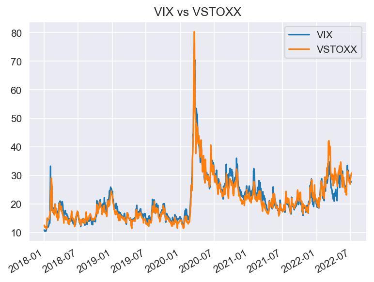
Despite their differences, extensive literature has shown that the two indices provide a valuable tool to understand market sentiment given the relevant negative correlation between the equity indices and their respective volatility indices:
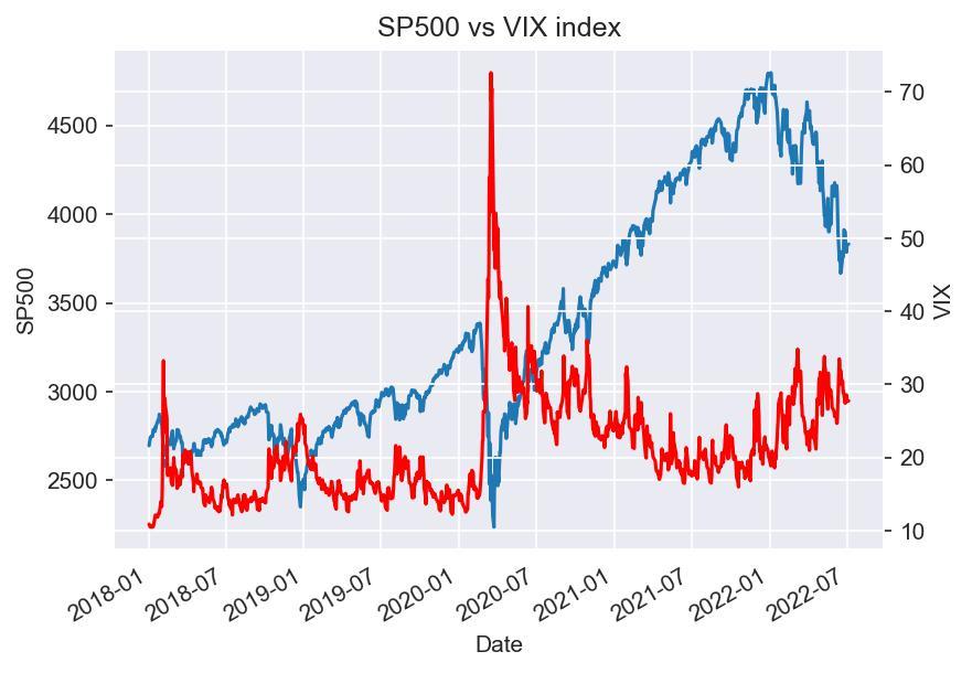
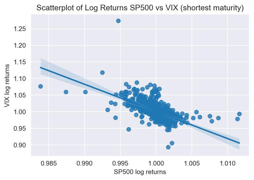
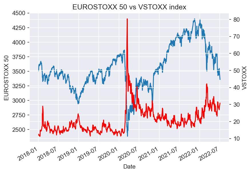
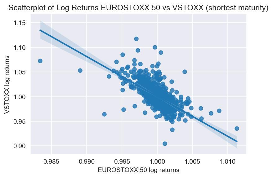
Source: Bocconi Students Investment Club
This phenomenon can be explained, at least partially, by the so-called “leverage effect”: indeed, given a fall in equity prices, the company’s leverage increases, thus increasing the risk for equity holders and therefore volatility, with the opposite also being true. As will be discussed in the section on the econometric model, the two effects on volatility tend to be asymmetric, with a higher impact on volatility stemming from negative shocks. Such a negative correlation makes the two volatility indices a valuable and desirable hedging tool for market participants, substantially increasing the volume growth of volatility derivatives.
It is not possible to invest in the indices themselves, however, meaning that one has to use derivatives, such as futures, which will be the focus of our article.
Moreover, as we can empirically verify, the two nearest term futures tend to exhibit a strong correlation, hinting at the stationarity of the spread between the two (which is not necessarily true for longer maturities):
Source: Bocconi Students Investment Club
This can also be statistically verified through the Augmented Dickey-Fuller (ADF). This test rejects the null hypothesis of a unit root in the spread time series at the 99%-confidence level.
A Vanilla Strategy
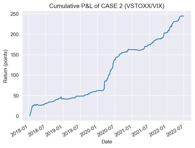
Our first trading strategy involves opening a short position on the higher index future and a long position on the lower one whenever the spread between VIX and VSTOXX surpasses 3% and closing our position whenever the spread reaches 1% (which has empirically proven to be the most profitable signal combinations).
It is important to mention that our back test runs on closing prices of the shortest maturity futures contract for each index, taking also into account the P&L that comes from the necessity to roll over to next maturity contracts whenever our trade is not closed within the maturity of the futures. Moreover, we consider the P&L arising from the opening of one long/short position for the VIX and 10 for the VSTOXX, as the multipliers are x1000 and x100, respectively, so as to have matching sensitivities. Yet, the data displayed below will report the profit and loss in indices points, rather than in currency amount.
Furthermore, it is worth mentioning that we do not take into account transaction costs, as empirical evidence suggests high levels of liquidity of the abovementioned futures contracts, and for the sake of simplicity we do not mention margin requirements in our analysis, which are determined by the exchanges as the sum of two main components: a marked-to-market requirement based on the current price of the underlying plus a risk mark-up defined by each exchange (CME for VIX futures and EUREX for VSTOXX).
As the data suggests, the spread trade yields positive profits both in the case of the VIX being higher and the VSTOXX lower, and in the opposite scenario (adjusting the trade position accordingly), as the two indices ultimately tend to converge.
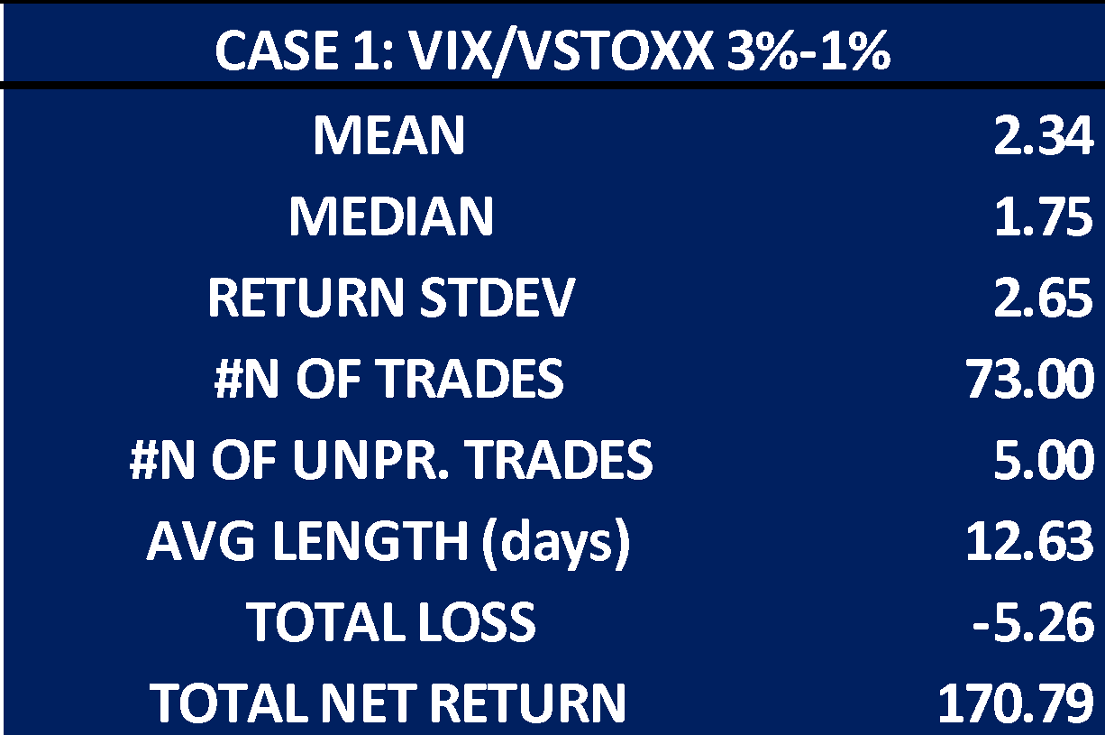
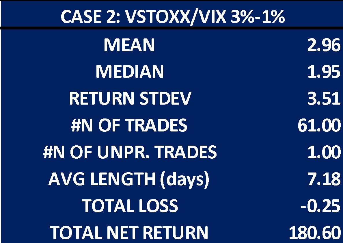
Source: Bocconi Students Investment Club
The data above shows some key highlights of the two “vanilla” trading strategies, where all relevant summary statistics, as well as the final P&L are in indices points. These quantities therefore have to be multiplied by 1000 (not taking into account currency exchange costs, given that the contracts are provided by different exchanges which are denominated in dollars and euros, respectively). Moreover, it is trivial that the two “cases” only apply the signal in one direction (VIX above VSTOXX and VSTOXX above VIX respectively) but given the nature of the trade itself we cannot have overlapping trades, thus making our theoretical P&L for the entirety of our “vanilla” strategy the sum of the two.
It is often the case, however, that when the trade closes in one direction it might be because the two indices have inverted, thus calling for the opening of the opposite position. Yet, if the strategy was put into place, such signals could also be observed intraday, thus not necessarily calling for the two operations to be done simultaneously.
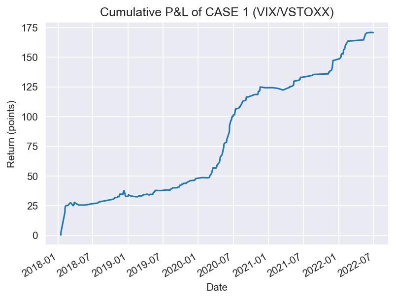
Source: Bocconi Students Investment Club
Moreover, as the above graphs show, it is interesting to notice that, although generally speaking the two strategies proved to be consistently profitable, some losses are to be expected: in particular, longer periods of consistently higher volatility in one of the two markets caused by “not globalized” systemic shocks could cause the spread to stay above our closing signal on either of the two sides for longer periods of times, causing us to roll futures several times, thus hurting the profitability of the trade. On the other hand, extreme shocks that eventually spread between markets, such as the COVID-19 crisis do constitute the perfect environment for our strategy to perform incredibly well.
A Brief Introduction to Risk Modeling
While time series models for the first moments of financial data (i.e. mainly returns) have been employed for a long time, only in the 1980s researchers moved to models for higher orders. This need arose due to the peculiar statistical properties of financial data.
First, the distribution of returns cannot be captured by normal distributions. Rather, the time series commonly display a leptokurtic structure, meaning that extreme observations as well as returns close to the mean are much more common than predicted by a normal distribution. Second, higher moments of returns (i.e. variances and covariances) are characterized by clusters. This is called conditional heteroskedasticity and captures the fact that large returns of either sign usually do not occur independently of each other but are more likely if another large move occurred in the previous period. Finally, as already mentioned above, the leverage effect is especially relevant when analyzing equity returns. Negative returns are expected to have a more pronounced impact on volatility since they lead to an increase in the debt-to-equity ratio of the company, worsening the risk profile.
These observations lead to the development of ARCH and GARCH models. For these models, it is first necessary to define a conditional mean model, usually based on an ARMA(p,q) structure. The first moments of the time series are therefore modeled as being dependent on p autoregressive lags and q white noise disturbances. The optimal lag length for both p and q are determined by Information Criteria (ICs) and the model is estimated by Maximum Likelihood (ML). A GARCH(1,1) model employs the error terms ε from the conditional mean model in the following way:
![]()
The variance forecast is therefore dependent on the squared error from the conditional mean model and the most recent variance forecast itself. GARCH(1,1) models are attractive due to their simplicity, while their forecasting power has also been shown to be strong, even when compared to more complex approaches. For reasons of simplicity, we leave out a discussion of stationarity conditions and the interpretation of the coefficients here and refer interested readers to the respective literature.
While GARCH models have been shown to be successful in accounting for conditional heteroskedasticity and leptokurticity, they fail to account for asymmetric effects on volatility. This is due to the fact that the model employs squared residuals, thereby eliminating any information stemming from the sign of mean model residuals. A broad variety of extensions of this model can account for these asymmetries. In the following, we briefly describe EGARCH and GJR-GARCH models as examples. These can be written as:

The models capture asymmetric impacts through different parameters. The EGARCH model comprises both the untransformed and absolute values of the errors, allowing for varying impacts depending on the sign. In the GJR-GARCH model, the indicator function discriminates between positive and negative shocks.
Defining a Dynamic Trading Strategy
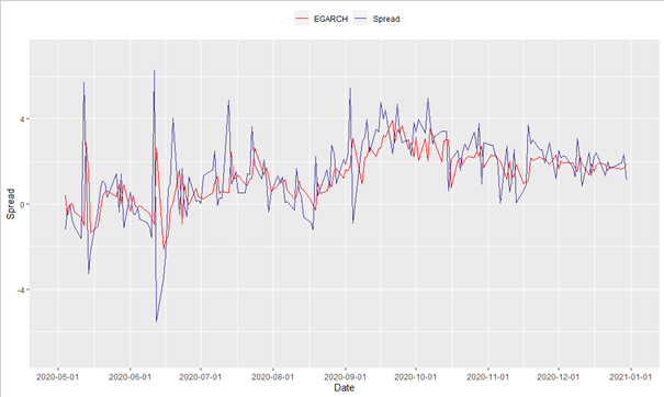
To find the best performing econometric model, we employ the following strategy. Using two years of daily data, every ten business days, we search the best performing conditional mean model. This process is done to account for the instability of the spread time series and based on the Akaike Information Criterion. As described above, the (squared) error terms of this model are then fed into the following three GARCH models: GARCH (1,1), EGARCH (1,1) and GJR-GARCH (1,1). The chart below shows the one-step ahead predictions of the EGARCH (1,1) model for the year 2020. For reasons of simplicity the other models were left out here and the time series was truncated.
Source: Bocconi Students Investment Club
Comparing the forecasting power of the employed models using mean-squared forecasting errors of the one-step ahead predictions of the spread, one obtains very similar results for all specifications. The values for the GARCH, EGARCH, and GJR-GARCH models are 2.88, 2.92 and 2.87, respectively. This similar performance of the symmetric GARCH model compared to the EGARCH and GJR-GARCH could be an indicator that the leverage effect has a less important role when predicting the spread between volatilities compared to the forecasting of outright levels.
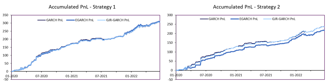
We employ two trading strategies to assess the profitability of systematic trading strategies over the considered time period:
- A simple strategy in which a spread position is opened every day. If the GARCH model predicts that the VIX-VSTOXX spread is going to widen compared to yesterday’s closing level, we enter a long spread position while a short spread position is opened if the GARCH forecast is lower than the current spread.
- To reduce the number of trades but potentially increase the confidence level in the prediction, we define an alternative strategy in which a long/short position is only entered if the difference between the current spread level and the one-step ahead forecast is bigger than a predefined number of estimation standard errors.
The charts below display the profit and losses for both types of strategies when employed during the time period from January 2020 to July 2022. For the second strategy, a threshold of 0.5 standard deviations was selected. An increase in this threshold would decrease the trading frequency.
Source: Bocconi Students Investment Club
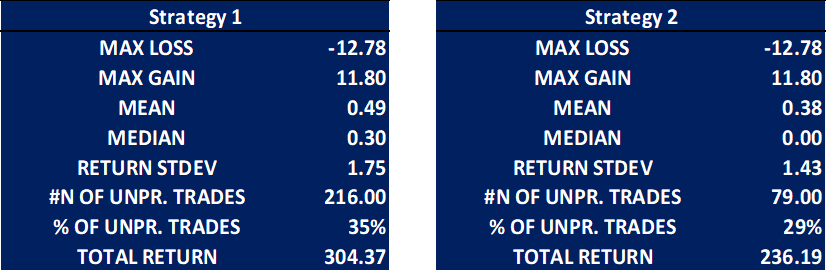
As anticipated, the second strategy reduces the number of transactions (and thus transaction costs) as well as the overall risk profile of the strategy. As above, the profit and loss in these charts is quantified by index points. The small differences in the time series between the employed GARCH models further confirms the fact that the different specifications are similar in their performance of predicting the index spread. The tables below summarize the performance of both strategies. For both strategies, the simplest model, i.e. GARCH (1,1) is used.
Source: Bocconi Students Investment Club
Conclusion
In this article, we introduced the VSTOXX and the VIX Indices as well as their respective future markets as hedging and investment tools. Further, we described the econometric challenges in modeling higher order moments of financial time series. Finally, we showed how different systematic trading strategies could be set up to trade the spread between the European and American implied volatility index.


3 Comments
steve xu · 26 January 2023 at 22:17
hi team. thanks for that. so which strategy has the higher sharpe? is the the mean reversion one or the GARCH model one pls?
Jay Urbain · 4 February 2023 at 20:13
Nice work. Is your code available? Thanks.
Luiz Beltreschi · 14 May 2023 at 18:18
Interesting paper. You do mention that the back test for the vanilla strategy runs on closing prices for the shortest futures on both VIX and VSTOXX. However, those markets close at different times. There are multiple circumstances when VSTOXX futures have already settled, but VIX futures have not. So even though VSTOXX futures will still be trading at, say, 3pm ET, the closing price for that day can be quite different. My question is: did you adjust the prices to reflect the same cut off time for both futures? Because if you did not, then you are trading with prices taken at different snapshots in time, and the results will not be realistic. Thank you.